What is Grey Wolf Optimization (GWO)?

Grey Wolf Optimization (GWO) is a nature-inspired, population-based metaheuristic proposed in 2014 by Seyedali Mirjalili and colleagues. It models the social hierarchy and hunting strategy of grey wolves (Canis lupus) to search for optimal or near-optimal solutions to complex optimization problems. In GWO, each candidate solution is a “wolf.” The pack collectively hunts a “prey” (the optimum) by encircling, exploring, and exploiting the search space. The algorithm’s elegance comes from two ideas:

• Leadership hierarchy: A small set of best solutions—α (alpha), β (beta), and δ (delta)—guide the entire pack (the remaining ω, or omegas).
• Hunting mechanics: Wolves update their positions by “encircling” the prey; mathematically, they follow the top three leaders and converge toward the promising region.

GWO has become popular because it is simple, few-parameter, and surprisingly competitive across engineering design, feature selection, scheduling, and machine learning hyperparameter tuning.

Introduction to the Grey Wolf Optimization Algorithm

Wolf’s exhibit coordinated hunting: tracking, encircling, and attacking prey. GWO abstracts these behaviors into search operators that alternate between exploration (broad search, finding promising regions) and exploitation (fine-grained search around promising regions).

• Population: A set of solutions (wolves) in a D-dimensional space.
• Fitness: The quality of each wolf’s solution according to a user-defined objective (to minimize or maximize).
• Leaders: The three best wolves are labeled α (best), β (second), and δ (third). They estimate the prey’s position.
• Fighters (ω): The rest of the wolves follow the leaders to update their positions.

Control is governed by a parameter a that linearly decreases from 2 to 0 over iterations. Large |A| (>1) encourages exploration; smaller |A| (<1) encourages exploitation. This smooth transition from roaming to converging makes GWO robust and easy to tune.

The Detailed GWO Algorithm

3.1 Encircling Prey

Grey wolves encircle prey before attacking. The encircling behavior in GWO is modeled as:

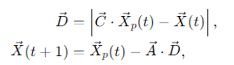
Where:

• X⃗p(t) is the prey’s position (unknown; approximated by leaders),
• X⃗(t) is the current wolf position,
• A⃗ and C⃗ are coefficient vectors:

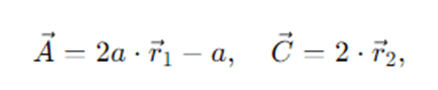
With r⃗1,r⃗2∼Uniform(0,1)D. The scalar a decreases linearly from 2 to 0 across iterations.

Intuition: C⃗ perturbs the prey estimate (diversity), while A⃗ controls how aggressively wolves move toward or around it. As a→0, wolves commit to exploiting the leaders’ region.

3.2 Leadership and Hunting

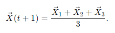
The actual prey location is unknown, so GWO estimates it via α, β, and δ—the three best solutions so far. Each wolf updates its position relative to each leader and averages the guidance:

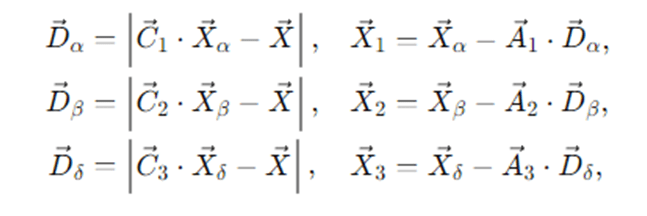
then

This triple-leader mechanism reduces bias and stabilizes convergence, because wolves do not chase only one leader’s potentially noisy estimate.

3.3 Exploration vs. Exploitation

• When ∣A⃗∣>1, the next position is pushed away from the leader—encouraging exploration.
• When ∣A⃗∣<1, wolves close in on the leader—favoring exploitation.

The linear schedule a↓0 moves the search from exploration to exploitation, much like simulated annealing’s cooling.

3.4 Boundary Handling

After each update, each dimension may be clamped to the feasible range [Lj,Uj]. Common strategies:

• Clamping: Xj←min⁡(max⁡(Xj,Lj).
• Reflection or random re-initialization (less common in basic GWO).

3.5 Stopping Criteria

Typical stopping criteria:

• Maximum number of iterations (or objective evaluations),
• Convergence threshold (fitness improvement below a tolerance),
• Time limit in time-critical applications.

Step-by-Step Explanation

• Initialize the pack: Begin by creating N wolves, each a D-dimensional vector sampled uniformly within the search bounds. Evaluate their fitness. Rank them and designate the top three as α (best), β (second best), and δ (third best). The remaining wolves are ω.
• Set control parameter a: Define a total of T iterations. Initialize a=2. At each iteration t∈{0,…,T−1}, update a←2−2⋅tT−1​. Early iterations therefore have larger a, enabling exploration; later iterations have smaller aaa, enforcing exploitation.
• Generate coefficient vectors A⃗,C⃗: For each wolf and each of the three leaders, generate fresh random vectors r⃗1,r⃗2∼U(0,1)D, then compute A⃗k=2ar⃗1−a and C⃗k=2r⃗2​ for k∈{α,β,δ}. These stochastic coefficients introduce diversity and prevent premature locking onto suboptimal regions.
• Compute three guidance positions: For each leader k∈{α,β,δ}, compute the distance vector D⃗k=∣C⃗k⋅X⃗k−X⃗∣ and the corresponding candidate position X⃗k′=X⃗k−A⃗k⋅D⃗k ​. Intuitively, each leader suggests where this wolf should move next relative to that leader.
• Average the guidance: Update the wolf’s position as the average of the three suggestions: X⃗←(X⃗α′+X⃗β′+X⃗δ′)/3. This triple averaging balances competing signals, smooths noise, and increases stability.
• Enforce bounds and evaluate: After updating all wolves, clip or reflect positions that leave the feasible region. Evaluate each wolf’s fitness at its new position.
• Refresh leaders: Re-rank the population by fitness. Update α, β, and δ if better wolves have emerged. Because leaders reflect the best-found positions to date, their guidance continually improves as the pack discovers better areas.
• Iterate until stop: Repeat steps 2–7 until the maximum number of iterations is reached or another stopping condition is satisfied. Return α as the best solution discovered, optionally along with its fitness, β, δ, and the pack history.

This cycle naturally mimics wolves’ behavior: start wide, scout multiple directions, then tighten the circle around the most promising region, guided by the three strongest hunters.

Pseudocode of GWO

Input: objective f, bounds [L,U], population size N, iterations T

Initialize wolves {X_i} ~ Uniform(L,U)

Evaluate {f(X_i)} and identify α, β, δ

for t = 0 to T-1:

    a = 2 – 2*(t/(T-1))

    for each wolf i:

        for leader k in {α, β, δ}:

            r1, r2 ~ U(0,1)^D

            A_k = 2*a*r1 – a

            C_k = 2*r2

            D_k = |C_k * X_k – X_i|

            X_k’ = X_k – A_k * D_k

        X_inew = (X_α’ + X_β’ + X_δ’) / 3

        X_inew = clamp(X_{i_new}, L, U)

    Replace {X_i} with {X_{i_new}}

    Evaluate {f(X_i)}; update α, β, δ

return α

Example: How GWO Works

5.1 Objective

Consider minimizing the 2D Sphere function:

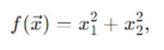
With bounds x₁, x₂∈[−5,5]. The global minimum is at (0,0) with f=0.

Assume a small pack of N=6 wolves for illustration. Initialize them randomly:

• W₁=(3.0,−4.0), f=25
• W₂=(−1.2,4.5), f≈22.1.22+4.52=1.44+20.25=21.69

(Let’s keep rounded values.) Say f≈21.7

• W₃=(2.8,0.5), f≈8.09
• W₄=(−3.6,−1.8), f≈16.2
• W₅=(0.6,−2.2), f≈5.0.36+4.84=5.20

(Say f≈5.2)

• W6=(−0.9,1.0), f≈1.81

Ranking by fitness (lower is better):

α = W6​ (1.81), β = W5​ (≈5.2), δ = W3​ (≈8.09). Others are ω.

Now, for each ω (and even leaders themselves in practice), compute three guidance moves from α, β, δ using the equations above. Early on, a is close to 2, so ∣A⃗∣ will often exceed 1, driving exploration—wolves might leap around the plane, probing directions. As iterations proceed and a↓0, ∣A⃗∣<1 becomes more common, and wolves start closing in around the triple-leader centroid, which is already near the origin because α, β, and δ are relatively close to (0,0).

Over, say, 50–200 iterations, you’ll see most wolves spiral toward the origin, with α improving repeatedly until it reaches a point extremely close to (0,0). On smooth convex problems like Sphere, GWO converges reliably; on rugged landscapes, it continues to juggle exploration and exploitation, often finding strong near-optima.

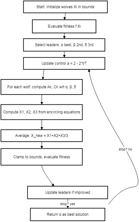
Algorithm Flow of GWO

Advantages and Disadvantages of GWO

Advantages

• Simplicity & few parameters: Only population size and iterations are mandatory; aaa is scheduled automatically.
• Balanced search: The aaa schedule and ∣A⃗∣|\vec{A}|∣A∣ threshold naturally transition from exploration to exploitation.
• Triple-leader guidance: Averaging α, β, δ reduces sensitivity to any single noisy guide and improves stability.
• General-purpose: Works well on continuous, nonconvex, multimodal problems; straightforward to hybridize with local search.
• Easy to implement & parallelize: Fitness evaluations can be parallelized; vectorized implementations are concise.

Disadvantages

• No guarantees of global optimality: Like most metaheuristics, convergence to the global optimum isn’t guaranteed.
• Sensitive to scaling & bounds: Poorly chosen ranges can slow convergence; normalization helps.
• Potential premature convergence: On deceptive landscapes, the pack may narrow too early; restart strategies or diversity control help.
• Hyperparameter choices still matter: Population size, iterations, and (if customized) aaa scheduling influence performance.
• Performance varies by problem: No free lunch—always benchmark against alternatives (PSO, DE, GA, CMA-ES, etc.).

Applications of GWO

• Machine learning & data mining: Feature selection, wrapper-based selection with classifiers (SVM, RF), hyperparameter tuning for neural networks, SVMs, and ensembles.
• Engineering design: Structural sizing, truss optimization, antenna array synthesis, power system stabilization, controller tuning (PID, fuzzy controllers).
• Signal & image processing: Multilevel image thresholding, image segmentation, filter parameter tuning, image registration.
• Scheduling & logistics: Task scheduling, load balancing in cloud/fog/edge computing, vehicle routing approximations.
• Cybersecurity: Attack detection threshold optimization, IDS parameter tuning, key feature selection in malware classification.
• Medical/healthcare analytics: Feature selection for diagnostic models, parameter estimation in physiological models.
• Renewable energy: Maximum power point tracking (MPPT) in PV systems, inverter/controller parameter optimization, wind turbine layout design.
• Finance & economics: Portfolio optimization (risk-return tradeoffs), calibration of models, technical indicator tuning for trading strategies.
• Control & robotics: Path planning, waypoint optimization, controller gains for UAVs and mobile robots.

Conclusion

Grey Wolf Optimization captures core aspects of collective intelligence: leadership, cooperation, and adaptive pressure between exploration and exploitation. Its success stems from (a) a minimalist design—easy to implement and tune—and (b) a triple-leader mechanism that stabilizes guidance while keeping diversity through random coefficients. In practical terms, GWO is a trustworthy baseline in continuous optimization and a solid building block for hybrid methods: attach a local search for fine polishing, inject restarts to fight stagnation, or co-evolve parameters for self-adaptation. While there is no one-size-fits-all optimizer, GWO’s blend of simplicity and performance makes it a must-try method for engineering design, ML hyperparameter tuning, and real-world decision systems where gradients are unavailable or unreliable.

Frequently Asked Questions (FAQs)

How do I choose population size and iterations for GWO?

There’s no universal rule, but common starting points are 20–50 wolves with 100–500 iterations for moderate problems. Increase population for rugged, high-dimensional landscapes; extend iterations if convergence plateaus near—but not at—acceptable fitness. Always validate with multiple random seeds.

What objective types can GWO handle?

Primarily continuous single-objective problems (minimization or maximization). With modifications, GWO can handle discrete/combination encodings (using rounding or problem-specific moves), multiobjective formulations (e.g., MOGWO), and constrained optimization (penalties, repair heuristics).

How do constraints fit into GWO?

Use penalty functions to augment the objective when constraints are violated, or apply repair/projection operators after position updates. Some applications incorporate feasibility rules or separate ranking (feasible first, then fitness).

How does GWO compare to PSO, DE, GA, or CMA-ES?

GWO often matches PSO and DE on many problems with less tuning effort. GA is flexible but may need more parameter tuning (crossover/mutation). CMA-ES excels on smooth, continuous problems—especially ill-conditioned—but is more complex. Best practice: benchmark several algorithms on your specific task.

 How can I avoid premature convergence?

Try larger populations, random restarts, adaptive or nonlinear aaa schedules, chaotic maps for r⃗1,r⃗2 ​, hybridizing with local search, or diversity preservation (e.g., mutation-like perturbations). Monitoring diversity (e.g., population variance) can trigger diversification when needed.