What is ResNet Algorithm?
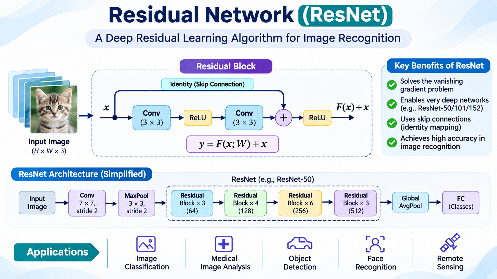
A Residual Network (ResNet) is a deep convolutional neural network architecture designed to train very deep models more effectively by introducing shortcut connections, also called skip connections. Instead of requiring a stack of layers to learn a complete mapping from input to output, a residual block learns a residual function with respect to its input. The block then adds the original input to that learned residual. This simple identity shortcut improves the flow of information and gradients through the network and makes it easier to optimize architectures containing dozens or even hundreds of layers.
In a conventional feed-forward network, each layer transforms the representation received from the previous layer. As the network becomes deeper, optimization can become difficult. The training accuracy may degrade as depth increases, even when overfitting is not the main cause. This is known as the degradation problem. ResNet addresses this issue using an identity shortcut that allows information to pass across one or more weight layers. A residual block can be represented as:
Residual transformation + identity shortcut
Here, x is the input feature representation, F(x,W) is the residual function learned by convolutional and other layers with parameters W, and y is the block output before its activation. When dimensions differ, a projection shortcut is used to align the input and residual dimensions. ResNet is widely used in image classification, object detection, segmentation, medical-image analysis and transfer learning.
Introduction to the ResNet Algorithm
Deep learning has achieved strong results in computer vision by using convolutional neural networks (CNNs) to learn hierarchical image representations. Early CNN architectures demonstrated that deeper feature extractors could improve recognition, but simply adding layers does not guarantee better performance. Very deep networks can be harder to train because signals and gradients must pass through many transformations. The problem is not only the traditional vanishing-gradient issue; deeper plain networks can also exhibit higher training error than shallower counterparts.
ResNet was introduced by Kaiming He and colleagues in the 2015 paper Deep Residual Learning for Image Recognition. Its central insight is to reformulate the desired mapping as a residual function. Suppose a few stacked layers should approximate a target mapping H(x). A plain design asks those layers to learn H(x) directly. A residual design instead learns F(x) = H(x) − x, then produces H(x) = F(x) + x. If the identity mapping is optimal, the residual branch can approach zero while the shortcut carries the input forward.
This formulation makes identity mappings easier to represent and provides a direct path for backpropagated gradients. The shortcut connection does not necessarily contain trainable parameters. In the basic form it is an identity operation; in projection blocks it uses a learned 1×1 convolution to match feature dimensions. ResNet variants include ResNet-18, ResNet-34, ResNet-50, ResNet-101 and ResNet-152. The shallower variants commonly use basic two-convolution blocks, whereas deeper variants such as ResNet-50 use bottleneck blocks containing 1×1, 3×3 and 1×1 convolutions.
A typical ResNet image-classification model begins with a convolution and pooling operation, proceeds through several residual stages at progressively different spatial resolutions, then applies global average pooling and a fully connected classification layer. The exact number of blocks, channels, normalization layers and downsampling locations depends on the selected ResNet variant and implementation.
Detailed Residual Network (ResNet) Algorithm
Step 1: Input image preparation
Let a batch of input images be represented by X ∈ RN×C×H×W, where N is the batch size, C is the number of channels, H is image height and W is image width. Images are decoded, resized or cropped to the required spatial dimensions, converted to tensors and normalized. For channel c, a common normalization is:
Here μc and σc are the training-set channel mean and standard deviation. Data augmentation such as random cropping, horizontal flipping and color transformations may be applied during training.
Step 2: Initial feature extraction
The input passes through a convolutional stem, often followed by batch normalization, a nonlinear activation and pooling. A convolution computes local feature responses:
The indices identify input channels, kernel positions and output feature maps. Padding and stride determine the output spatial dimensions. Batch normalization stabilizes intermediate activations, and ReLU introduces non-linearity: ReLU(z) = max(0,z).
Step 3: Residual block transformation
The central operation of ResNet is the residual block. For input x, a residual branch applies a sequence of transformations, such as convolution, normalization and activation. The resulting function is F(x,W). A simplified two-layer basic block can be expressed as:
This expression is illustrative; implementations commonly place batch normalization and activations around each convolution according to the block design. The residual and shortcut paths are combined by element-wise addition:
Basic identity residual block
The addition requires the tensors to have compatible dimensions. The shortcut preserves the input signal while the residual branch learns an adjustment to it.
Step 4: Dimension matching with projection shortcuts
At stage transitions, feature-map channels or spatial resolution can change. In that case, x cannot be added directly to F(x,W). ResNet uses a projection shortcut, often a 1×1 convolution with a suitable stride:
Ws represents the projection parameters. A 1×1 convolution changes the channel dimension, while its stride can reduce spatial resolution. The projection is selected to make the shortcut output match the residual branch shape.
Step 5: Bottleneck residual block
Deeper ResNet models such as ResNet-50 use a bottleneck design to reduce computation. It first uses a 1×1 convolution to reduce channels, then a 3×3 convolution to process spatial information, and finally a 1×1 convolution to expand channels. A simplified formulation is:
The symbol * denotes convolution, and the equation omits some implementation-specific normalization and activation placements for clarity. The bottleneck reduces the cost of the middle 3×3 convolution while allowing a wider output representation.
Step 6: Build multiple residual stages
The network stacks residual blocks into stages. Within a stage, blocks generally preserve the same feature-map dimensions. The first block of a new stage may reduce spatial resolution and increase channel count, using a projection shortcut when required. Later stages represent increasingly abstract patterns, from edges and textures to object parts and semantic concepts. ResNet depth refers to the number of weighted layers, not the number of residual blocks alone.
Step 7: Global average pooling
After the final residual stage, a feature tensor A ∈ RC×H×W is converted into a compact vector through global average pooling:
This operation averages each channel over its spatial positions, producing one feature value per channel and reducing the number of classifier parameters.
Step 8: Classification layer and probability
The pooled feature vector is passed to a fully connected layer that produces class logits:
For K classes, softmax converts the logits into probabilities:
The predicted class is argmaxk pk. For multi-label tasks, independent sigmoid outputs and a suitable binary loss are often used instead of softmax.
Step 9: Loss calculation
For a single-label classification problem with one-hot target y, categorical cross-entropy is:
For a batch of N samples, the average data loss is Lbatch = (1/N)ΣnLn. Regularization such as weight decay may be added to the objective.
Step 10: Backpropagation through residual connections
Training computes gradients of the loss with respect to all trainable parameters. For a block y = F(x,W) + x, the derivative with respect to x includes a direct identity contribution:
For y = ReLU(F(x,W)+x), the derivative also includes the activation mask. The identity term provides a direct gradient route through the shortcut, although it does not eliminate every optimization challenge or guarantee that gradients never vanish or explode.
Step 11: Parameter update
An optimizer such as stochastic gradient descent (SGD) updates the model parameters. A basic update with learning rate η is:
Momentum, learning-rate schedules, weight decay and other optimizer settings can improve convergence. These choices should be selected using validation data rather than the final test set.
Step 12: Validation and inference
After each training epoch, the model is evaluated on validation data to monitor generalization and select checkpoints. At inference time, preprocessing is applied consistently, the trained network performs a forward pass, and the output probabilities or predictions are returned. No gradient computation or parameter update is required.
Step-by-Step Explanation
First, prepare the image dataset. Collect labeled images and divide them into training, validation and test partitions without allowing information from the test set to influence model development. Decode each image, standardize its size and normalize pixel values using statistics calculated from the training data. During training, augmentation may create varied views of the same image through crops, flips or mild color changes. The objective is to improve robustness while preserving the correct label.
Next, initialize the network architecture. Select an appropriate ResNet variant according to the dataset size, computational budget and target application. A small task may start with ResNet-18, while a larger or more demanding task may use ResNet-50 or a deeper model. The initial convolutional stem extracts low-level patterns. Batch normalization and ReLU stabilize and transform the activations, and pooling can reduce spatial dimensions before the residual stages.
Then, process each residual block. The block receives a feature tensor and sends it through its residual branch. Convolutional filters learn a transformation that emphasizes useful changes to the representation. At the same time, a shortcut carries the original tensor forward. The two paths are added element by element and passed through the activation specified by the architecture. This design allows a block to learn a refinement rather than having to reconstruct the entire desired feature mapping.
When tensor sizes differ, align the shortcut. The network checks whether the shortcut and residual outputs have the same number of channels and spatial dimensions. If they match, the identity is added directly. If a stage transition changes the resolution or channel count, a projection shortcut performs the required transformation. This dimension matching is essential because element-wise addition cannot combine tensors with incompatible shapes.
After the residual stages, summarize the learned features. Later blocks encode increasingly high-level structures. Global average pooling aggregates each feature map into a single value. The resulting vector is passed into a dense classification layer, which generates one score per target class. Softmax converts those scores to class probabilities for a mutually exclusive classification task.
Calculate the prediction error and update the weights. Cross-entropy compares predicted probabilities with the known labels. Backpropagation computes gradients through both the residual and shortcut routes. The shortcut provides a direct gradient contribution, helping information travel through the network. The optimizer uses these gradients to update convolutional filters, normalization parameters and classifier weights. Mini-batches are processed repeatedly over multiple epochs.
Finally, evaluate and deploy the trained model. Validation metrics guide decisions such as learning-rate adjustment, checkpoint selection and early stopping. Once the design is fixed, the test set is used for a final unbiased assessment. A deployed model uses the same preprocessing and class-index mapping as training. For practical applications, measure accuracy alongside latency, memory, throughput and robustness under realistic input conditions.
Example: How the Residual Network (ResNet) Algorithm Works
Consider an illustrative image-classification task that distinguishes between cats and dogs. A training set contains labeled examples from both classes. An image is resized and normalized, then passed through the ResNet stem. The early convolutional layers detect local visual patterns such as edges, corners and textures. Subsequent residual stages combine these patterns into more informative representations, including shapes, fur patterns, ears and object-level structures.
To understand the residual addition numerically, consider a simplified feature vector entering one residual block:
F(x,W) = [0.2, −0.5, 0.3]
Assume the dimensions match and the shortcut is an identity mapping. The block adds the two vectors:
y = [1.0 + 0.2, 2.0 − 0.5, 0.5 + 0.3] y = [1.2, 1.5, 0.8]
If the block applies ReLU after addition, all three values remain unchanged because they are positive. The output therefore retains the original information while incorporating the learned adjustment. The values above are illustrative, not measured outputs from a trained ResNet.
In a real classifier, the final pooled vector is transformed into two logits, for example z = [1.8, 0.9] for classes cat and dog. The softmax probabilities are approximately p(cat) = 0.711 and p(dog) = 0.289. The model predicts cat because it has the higher probability. If the correct label is cat, cross-entropy is −log(0.711), approximately 0.341. Training uses this loss to compute gradients and update the network parameters.
At a stage transition, suppose the residual branch produces a tensor with 128 channels at 28×28 resolution, while the incoming shortcut has 64 channels at 56×56. Direct addition is impossible. A 1×1 projection convolution with stride 2 can map the shortcut to 128 channels at 28×28. The two tensors then have compatible shapes and can be added. This illustrates how ResNet uses identity shortcuts in ordinary blocks and projection shortcuts when dimensions change.
In practice, model quality is evaluated on images not used for training. Useful measures include accuracy, precision, recall, F1-score and confusion matrix. For imbalanced datasets, per-class recall, macro-F1 and balanced accuracy can be more informative than overall accuracy alone.
The following simplified diagram shows the data flow inside a residual block. The input travels through a convolutional residual branch while a shortcut bypasses the transformation layers. Both paths meet at an element-wise addition operation.
Convolution
Batch Normalization
ReLU
Convolution
Batch Normalization
Identity mapping
(or 1×1 projection)
Residual block: y = ReLU(F(x,W) + x), or y = ReLU(F(x,W) + Wsx) with a projection shortcut.
A complete image-classification pipeline can be summarized as: input image → stem convolution and pooling → residual stage 1 → residual stage 2 → residual stage 3 → residual stage 4 → global average pooling → fully connected layer → class probabilities. ResNet-50 uses bottleneck blocks in its residual stages; the number of blocks per stage depends on the model variant.
Pseudocode for the Residual Network (ResNet) Algorithm
Algorithm: Train a Residual Network for Image Classification

Input:
    Training dataset Dtrain
    Validation dataset Dval
    Number of classes K
    ResNet architecture (e.g., ResNet-50)
    Epoch count E
    Learning rate η

Output:
    Trained ResNet model

1.  Initialize ResNet parameters W
2.  Define preprocessing and training-time augmentation
3.  For epoch = 1 to E:
4.      Set model to training mode
5.      For each mini-batch (X, Y) in Dtrain:
6.          Normalize and augment X
7.          A ← InitialStem(X)
8.          For each residual block B in the network:
9.              R ← ResidualBranch(A, B.parameters)
10.             If shortcut dimensions match:
11.                 S ← A
12.             Else:
13.                 S ← ProjectionShortcut(A)
14.             A ← Activation(R + S)
15.         G ← GlobalAveragePooling(A)
16.         Z ← FullyConnected(G)
17.         P ← Softmax(Z)
18.         L ← CrossEntropy(P, Y)
19.         Compute gradients ∇W L by backpropagation
20.         Update W using optimizer and learning rate η
21.     Set model to evaluation mode
22.     Evaluate model on Dval without gradient updates
23.     Record validation loss and evaluation metrics
24.     Adjust learning rate / save best checkpoint as required
25. Return the best validation checkpoint
The pseudocode describes the main training logic rather than every implementation detail. Modern frameworks handle tensor operations, mixed precision, gradient scaling, distributed training and optimizer state. For reproducible experiments, record the architecture, input resolution, preprocessing, random seeds, optimizer settings, data split and software versions.
Advantages and Disadvantages of ResNet Algorithm
Advantages
- Improved optimization of deep networks: Shortcut connections make identity mappings easier to learn and provide a direct route for gradient flow.
- Supports greater depth: ResNet architectures can be built with many layers while remaining practical to optimize compared with corresponding plain networks.
- Strong visual representations: Residual stages learn hierarchical features that are useful for many computer-vision tasks.
- Transfer learning: Pretrained ResNet weights can be fine-tuned or used as feature extractors for specialized datasets.
- Flexible architecture: Multiple depths and block designs make it possible to balance accuracy and computation.
- Broad ecosystem support: ResNet implementations and pretrained checkpoints are available in popular deep-learning frameworks.
Disadvantages
- Computational cost: Deep variants require substantial processing time, memory and energy, particularly at high image resolutions.
- Large training datasets: Training from scratch can require many labeled images and careful regularization to generalize well.
- Hyperparameter sensitivity: Learning rate, batch size, weight decay and augmentation choices can materially affect convergence.
- Deployment constraints: Some variants may be too large or slow for low-power devices without pruning, quantization or other optimization.
- Limited task-specific reasoning: A standard ResNet classifier does not automatically provide object localization, segmentation or explanations; task-specific heads and methods are needed.
- Shortcut complexity at transitions: Projection shortcuts and stage changes add design choices and must be implemented with correct tensor dimensions.
Consequently, the best ResNet configuration depends on the task, dataset, target hardware and accuracy requirements. A very deep model is not always the best model for a small dataset or latency-sensitive deployment.
Applications of the ResNet Algorithm
Image classification: ResNet is widely used to assign images to categories, such as animals, vehicles, plants, products and everyday objects. Pretrained networks provide strong starting points for transfer learning.
Object detection: Residual networks can act as backbone feature extractors in detection frameworks. The extracted multi-level features help detection heads identify object categories and bounding boxes.
Image segmentation: ResNet backbones are frequently incorporated into encoder-decoder segmentation systems. They support pixel-level tasks such as road-scene understanding, land-cover mapping and lesion delineation.
Medical image analysis: ResNet-based models have been investigated for classifying radiographs, retinal images, MRI scans, CT images and histopathology images. Clinical deployment requires rigorous validation, careful handling of patient-level data splits, bias analysis and appropriate clinical oversight.
Remote sensing and satellite imagery: Residual feature extractors support land-use classification, crop monitoring, building recognition, disaster assessment and change detection using aerial or satellite images.
Industrial inspection: Manufacturing systems can use ResNet models to classify surface defects, identify damaged components and support automated quality-control workflows. Performance should be tested across different lighting, cameras and production conditions.
Face and person analysis: ResNet-derived architectures have been used as feature extractors in face-related and person-recognition research. Such applications require special attention to privacy, fairness, consent and applicable laws.
Video analytics: ResNet can extract frame-level visual features that are combined with temporal models or video transformers for action recognition, event analysis and surveillance research.
Scientific image analysis: Researchers apply residual architectures to microscopy, cell classification, material characterization and astronomical image categorization. Fine-tuning can adapt pretrained representations to domain-specific image distributions.
Conclusion
The Residual Network (ResNet) algorithm is an influential deep-learning architecture that improves the training of deep convolutional neural networks through residual learning and shortcut connections. By learning a residual transformation and adding the input through an identity or projection shortcut, each block can refine feature representations while maintaining a direct information path. This design addresses the degradation problem associated with simply increasing network depth and supports practical architectures such as ResNet-18, ResNet-34, ResNet-50, ResNet-101 and ResNet-152.
This tutorial explained the residual mapping equations, identity and projection shortcuts, bottleneck blocks, classification pipeline, backpropagation, a numerical example, a digital block diagram and training pseudocode. ResNet has broad applications in image classification, detection, segmentation, medical imaging, remote sensing and industrial inspection. Nevertheless, model selection should consider computational requirements, dataset quality, validation methodology, fairness and deployment constraints. When applied with sound experimental design, ResNet remains a useful baseline and feature-extraction architecture for computer-vision research and real-world systems.
Frequently Asked Questions (FAQs)
Q1. What is the main idea behind the ResNet algorithm?
ResNet uses shortcut connections so a block learns a residual function F(x) and adds the original input x, producing F(x) + x. This helps preserve information and improves optimization in deep networks.
Q2. What is a residual connection in ResNet?
A residual connection is a shortcut path that carries a block’s input directly to the addition operation. It is usually an identity mapping, but a projection such as a 1×1 convolution is used when dimensions must change.
Q3. What is the difference between ResNet-18 and ResNet-50?
They differ in depth and block design. ResNet-18 uses basic residual blocks, while ResNet-50 uses bottleneck blocks with 1×1, 3×3 and 1×1 convolutions. ResNet-50 is generally more computationally demanding.
Q4. Why does ResNet use skip connections?
Skip connections provide a direct information and gradient route across residual layers. They make identity mappings easier to represent and help reduce the degradation that can occur when plain networks become deeper.
Q5. Can ResNet be used for medical image classification?
Yes. ResNet can be trained or fine-tuned for tasks involving X-rays, MRI, CT, retinal and pathology images. Reliable medical use requires representative data, patient-level separation, external validation and clinical evaluation.
Q6. Is ResNet suitable for transfer learning?
Yes. A model pretrained on a large image dataset can be used as a fixed feature extractor or fine-tuned on a smaller target dataset. The preprocessing and normalization expected by the pretrained weights should be followed.
References
- He, K., Zhang, X., Ren, S., and Sun, J. (2016). Deep Residual Learning for Image Recognition. Proceedings of the IEEE Conference on Computer Vision and Pattern Recognition (CVPR), 770–778. https://doi.org/10.1109/CVPR.2016.90
- He, K., Zhang, X., Ren, S., and Sun, J. (2015). Deep Residual Learning for Image Recognition. arXiv preprint arXiv:1512.03385. https://arxiv.org/abs/1512.03385
- He, K., Zhang, X., Ren, S., and Sun, J. (2016). Identity Mappings in Deep Residual Networks. European Conference on Computer Vision (ECCV), 630–645. https://arxiv.org/abs/1603.05027
- Szegedy, C., Liu, W., Jia, Y., et al. (2015). Going Deeper with Convolutions. Proceedings of the IEEE Conference on Computer Vision and Pattern Recognition. https://arxiv.org/abs/1409.4842
- Goodfellow, I., Bengio, Y., and Courville, A. (2016). Deep Learning. MIT Press. https://www.deeplearningbook.org/
External Learning Resources
- PyTorch Torchvision: ResNet model documentation — architecture definitions and pretrained model interfaces.
- TensorFlow Keras: ResNet50 documentation — model loading and preprocessing details.
- Original ResNet research paper — research motivation, architecture and evaluation.
- Papers with Code: ResNet — related benchmarks and research implementations.