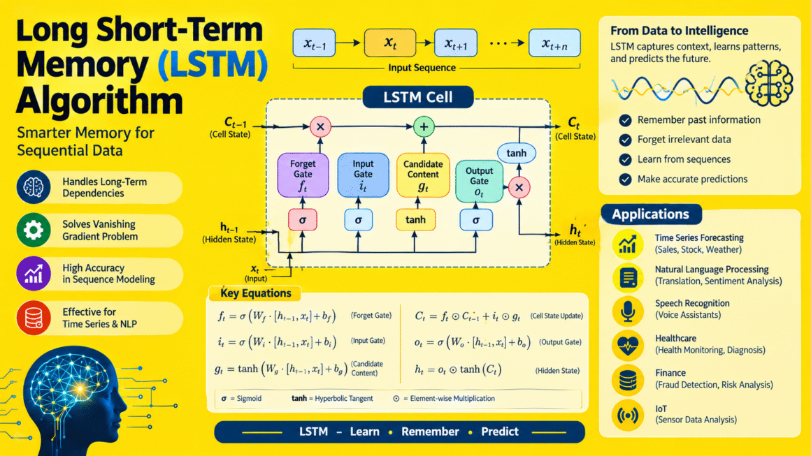
Long Short-Term Memory (LSTM) is a type of recurrent neural network (RNN) designed to learn patterns in sequential data while retaining useful information over time. Its distinctive memory cell and gating mechanisms help control what information is stored, updated, and exposed at each time step. LSTMs are widely used in time-series forecasting, language processing, speech recognition, anomaly detection, and other tasks where the order of observations matters.

This guide explains the LSTM algorithm, its mathematical operations, the roles of the input, forget, and output gates, a step-by-step training workflow, a worked example, a digital flow diagram, pseudocode, advantages, limitations, and applications. It also discusses how an LSTM learns through backpropagation through time (BPTT), how to prepare sequential data, and how to evaluate a model responsibly. The equations below describe a standard LSTM cell; practical implementations may vary in gate ordering, bias conventions, peephole connections, and other architectural details.

What Is the Long Short-Term Memory ?

Long Short-Term Memory is a gated recurrent neural network architecture introduced by Sepp Hochreiter and Jürgen Schmidhuber in 1997. It was developed to address limitations of ordinary recurrent neural networks, especially the difficulty of learning long-range dependencies during training. In a basic RNN, information is passed from one time step to the next through a hidden state. During backpropagation across many time steps, gradients can become extremely small or large, making it difficult to learn relationships separated by long intervals.

An LSTM adds a memory cell, often denoted c_t, alongside a hidden state h_t. Three gates regulate the flow of information: the forget gate determines what old memory to retain, the input gate controls how much new candidate information to write, and the output gate controls which memory information becomes visible in the hidden state. These gates are learned from data, so the model can adapt its memory behavior to the task.

At time step t, the cell receives the current input x_t, previous hidden state h_t−1, and previous cell state c_t−1. It calculates gate activations, updates its cell memory, and produces a new hidden state. For a sequence, this process repeats in order across all time steps while the same learned parameters are reused. The resulting hidden states can be used for next-step prediction, sequence classification, sequence-to-sequence modeling, or other objectives.

Introduction to the LSTM Algorithm

Sequential data appear in many fields: stock prices, weather observations, medical measurements, sensor readings, spoken audio, and natural-language text. In such data, an observation may depend not only on its current value but also on earlier events. For example, a demand forecast may depend on weekday patterns and previous sales, while a language model may need information from earlier words to interpret the current word.

Traditional feed-forward networks process a fixed input without an inherent recurrent state. A standard RNN introduces recurrence by updating its hidden state using the current input and previous hidden state. A simplified RNN update is h_t = tanh(W_xx_t + W_hh_t−1 + b). Although this structure can represent sequence dependencies, repeated multiplication through recurrent transitions can cause gradients to vanish or explode over long sequences. When gradients vanish, the model may fail to learn useful relationships between distant time steps.

LSTM addresses this issue by introducing a more controlled memory pathway. The cell state is updated through an additive combination of retained memory and new candidate content. The forget and input gates determine the relative contributions. This design creates a path through which information and gradients can flow across multiple steps more effectively than in a conventional RNN, although it does not eliminate all optimization difficulties or guarantee that every long-range dependency will be learned.

LSTM is a model architecture rather than a complete task-specific solution. The algorithm includes choosing an input representation, preparing sequences, defining the network and output layer, selecting a loss function, training the model, and evaluating generalization. For forecasting, the model may take a window of historical values and predict the next value or several future steps. For text classification, it may process token embeddings and use the final or pooled hidden representation to predict a label.

Detailed LSTM Algorithm

3.1 Define the sequence-learning problem

Let the input sequence be X = (x₁, x₂, …, x_T), where each x_t ∈ ℝ^d is a feature vector at time t. The model produces hidden states and predictions over the sequence. In a forecasting task, the objective might be to predict a target y_t+1 from the past observations. In sequence classification, the target may be one label for the complete sequence. Define the task, prediction horizon, input features, target variables, and loss before building the model.

3.2 Initialize parameters and states

An LSTM has trainable weight matrices and bias vectors for its gates and candidate cell content. For a hidden dimension H and input dimension d, each gate typically uses a combined input/recurrent weight matrix of shape H × (d+H), plus a bias vector of length H. The initial hidden state and cell state are commonly set to zero for each independent sequence, though learned initial states or stateful processing may be used in some applications.

Concatenate the current input and previous hidden state as z_t = [h_t−1, x_t]. This is a notational convenience; frameworks may store separate input and recurrent matrices instead. At each time step, the same parameter matrices are reused, which lets the model process sequences of different lengths subject to the chosen batching and masking strategy.

3.3 Forget gate

The forget gate controls how much of the previous cell memory is retained:

f_t = σ(W_f[h_t−1, x_t] + b_f)

The sigmoid function σ(a) = 1 / (1 + e^−a) maps values to the interval (0,1). A value near 1 means retaining more of the corresponding memory component; a value near 0 means forgetting more of it. The forget gate acts element-wise, so different dimensions of the cell state can retain or discard different information. The gate does not decide what is important through a hand-coded rule; its weights are learned during training.

3.4 Input gate and candidate cell content

The input gate controls how much new information should be written into memory:

i_t = σ(W_i[h_t−1, x_t] + b_i)

A candidate cell vector represents potential new content:

g_t = tanh(W_g[h_t−1, x_t] + b_g)

The tanh function maps its input to (−1,1), allowing positive and negative candidate values. The input gate scales the candidate content element-wise. This separation between deciding what to write and proposing what to write gives the cell more control than a simple recurrent update.

3.5 Update the cell state

The new cell state combines retained old memory with selected candidate content:

c_t = f_t ⊙ c_t−1 + i_t ⊙ g_t

Here, ⊙ denotes element-wise multiplication. The first term preserves part of the previous memory; the second term adds new information. This additive state update is central to LSTM’s ability to maintain information over longer sequences. If a forget-gate component remains near one and the input gate contributes little new content, the corresponding cell-state component can persist across time steps.

3.6 Output gate and hidden state

The output gate determines which parts of the memory are exposed as the hidden state:

o_t = σ(W_o[h_t−1, x_t] + b_o)

The hidden state is then calculated as:

h_t = o_t ⊙ tanh(c_t)

The hidden state is passed to the next time step and can also be used by the prediction layer. The cell state functions as an internal memory, while the hidden state is the gated representation exposed to the rest of the network. Both states are important, but they serve different roles in the computation.

3.7 Generate predictions

For a sequence classification task, the final hidden state or a pooled representation may feed a classifier. For example, logits can be calculated as z = W_yh_T + b_y, then converted to class probabilities using softmax. For binary classification, a sigmoid output may be used. For regression or forecasting, a linear output layer is common: ŷ_t+1 = W_yh_t + b_y. Sequence-to-sequence tasks may generate predictions at each time step or use an encoder-decoder design.

3.8 Define the loss function

The loss measures the difference between predictions and targets. For regression, mean squared error is commonly used:

L_MSE = (1/N) Σ_n=1^N(y_n − ŷ_n)²

Mean absolute error is another option and is less sensitive to large errors. For multi-class classification, cross-entropy is typical:

L_CE = −Σ_k y_k log(p_k)

The selected loss must match the task and output representation. For forecasting, the train/validation split should respect time order to prevent future observations from leaking into training. Scaling parameters should be fitted on the training data only.

3.9 Backpropagation through time (BPTT)

Training an LSTM requires calculating how the loss changes with respect to its shared parameters. Backpropagation through time unrolls the recurrent computation across sequence steps and applies the chain rule backward through the unrolled graph. Gradients from later predictions can influence parameters used at earlier time steps. For long sequences, full BPTT can consume substantial memory; truncated BPTT limits the number of steps through which gradients are propagated, trading computational efficiency against the ability to learn very long dependencies.

Although LSTM gates can improve gradient flow, gradients may still vanish or explode in some settings. Gradient clipping can limit unusually large gradient norms, and careful initialization, normalization, sequence length selection, and learning-rate tuning can improve stability.

3.10 Update parameters

After gradients are calculated, an optimizer updates model parameters. A basic gradient-descent update is:

θ_t+1 = θ_t − η∇_θL

where θ represents all trainable parameters and η is the learning rate. In practice, mini-batch stochastic gradient descent, Adam, or related optimizers are common. Training repeats the forward pass, loss calculation, backward pass, and parameter update over multiple mini-batches and epochs. Validation metrics help choose model settings and determine when training should stop.

3.11 Sequence batching and masking

Sequences often have different lengths. To batch them efficiently, implementations may pad shorter sequences and use masks or packed-sequence utilities so that padding does not affect the model’s learning or evaluation. For time-series windows, all samples may be created with a fixed look-back length. The model’s input shape commonly follows (batch, time steps, features), although frameworks can support other conventions.

3.12 Termination and model selection

Training may stop after a predefined number of epochs, when validation loss stops improving, or when a computational budget is reached. Save the best checkpoint according to a preselected validation metric. Evaluate the final model on a held-out test set only after model selection. For forecasting, report metrics such as MAE, RMSE, or MAPE when appropriate; MAPE requires care when actual values are zero or near zero. For classification, report metrics that reflect class imbalance and application costs.

 Explanation of the LSTM Algorithm

Step 1—Collect sequential data. Identify the time-dependent observations, input features, and target. Examples include hourly energy consumption, daily sales, patient vital signs, sensor signals, or tokenized text. Check timestamp consistency, missing values, duplicates, irregular sampling, and label quality. When the task is forecasting, keep the chronological order intact and avoid using information that would not be available at prediction time.

Step 2—Preprocess and create sequences. Handle missing values with a method suitable for the domain, scale numeric features using training-set statistics, and convert the data into sequences. A common sliding-window setup uses the previous L observations to predict the next H values. For instance, a look-back window of 24 hourly observations may predict the next hour or next several hours. Split the data before fitting scalers and creating leakage-prone transformations.

Step 3—Choose the LSTM architecture. Select the number of LSTM layers, hidden units, dropout, and output-layer design. A single LSTM layer may be enough for a small problem, while stacked layers can represent more complex patterns at higher computational cost. Bidirectional LSTMs process sequences in both directions and can be useful when the entire input sequence is available, such as offline text classification. They are generally unsuitable for causal forecasting if backward processing would use future values unavailable at prediction time.

Step 4—Initialize states and parameters. Initialize gate weights and biases using the framework’s supported methods or a carefully chosen initialization strategy. Set hidden and cell states to zero for independent sequences unless the application uses learned or carried-over states. For stateful streaming, reset or carry states consistently at sequence boundaries; otherwise, information can leak between unrelated examples.

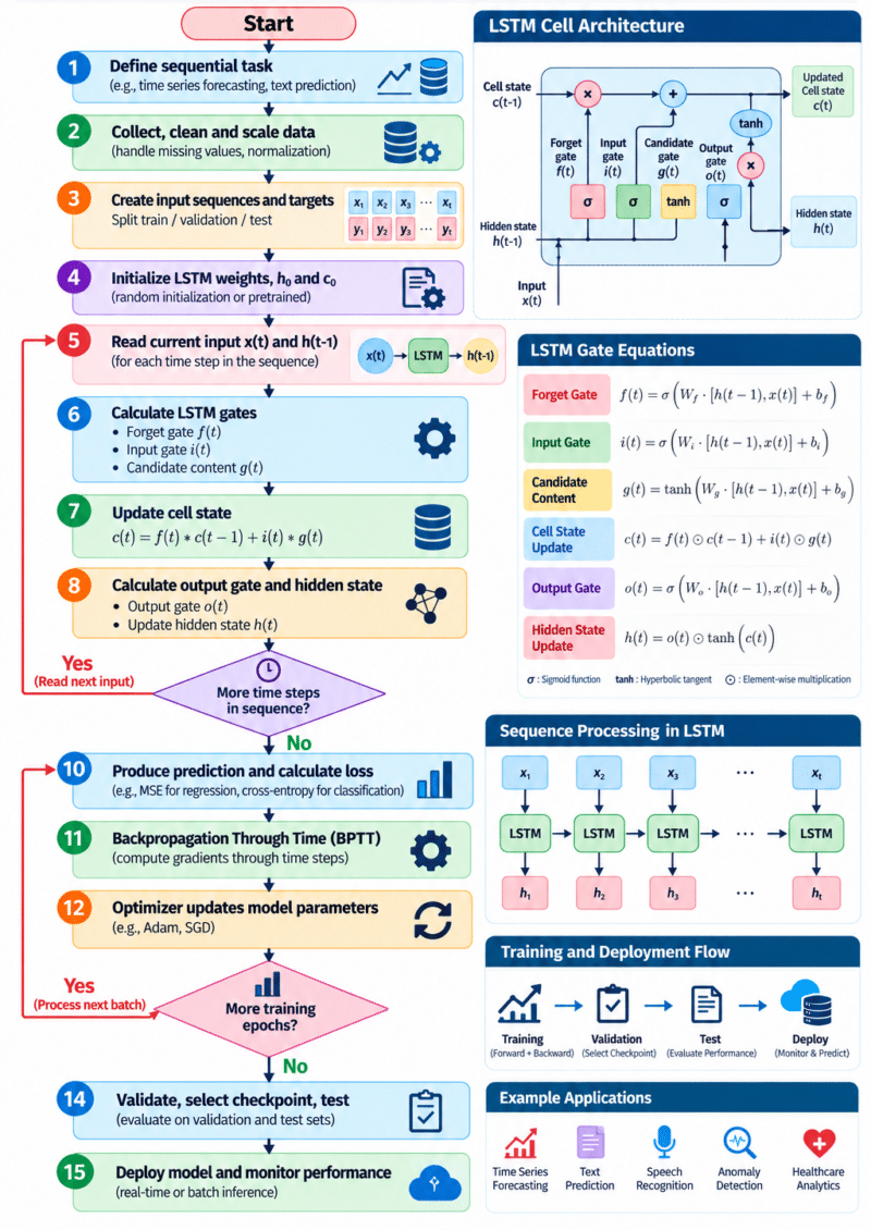
Step 5—Process each time step. The LSTM reads the current input vector and previous hidden state. It calculates the forget gate, input gate, candidate cell content, and output gate. These operations control how previous memory is retained, what new information is stored, and which memory components become visible. The cell state and hidden state are updated and passed forward to the next time step.

Step 6—Generate a prediction. Use the final hidden state, a sequence of hidden states, or a pooled representation according to the task. A classifier may predict a category, while a forecasting head may output one or multiple future values. The output dimensions, activation function, and target encoding must match the task being solved.

Step 7—Calculate the loss. Compare predictions with known training targets using the selected loss function. For regression, MSE or MAE is common; for classification, cross-entropy is frequently used. Aggregate the loss over the relevant samples or time steps, taking care to mask padded positions or ignored labels when needed.

Step 8—Backpropagate through the sequence. Use BPTT to calculate gradients through the recurrent steps and output layer. The gradients update the shared gate weights, recurrent weights, biases, and prediction-head parameters. For long sequences, consider truncated BPTT, gradient clipping, or smaller batches to manage memory and improve training stability.

Step 9—Update parameters and repeat. The optimizer adjusts the model parameters based on gradients. Repeat training over mini-batches and epochs, monitoring both training and validation losses. If training performance improves while validation performance worsens, the model may be overfitting; consider early stopping, regularization, smaller models, or more representative data.

Step 10—Evaluate and deploy. Restore the best validation checkpoint and assess it on held-out test data. Compare against simple baselines such as persistence forecasting, seasonal averages, logistic regression, or a standard RNN when appropriate. Document preprocessing, sequence length, prediction horizon, architecture, random seeds, and metrics. For deployment, verify inference latency, memory requirements, missing-data behavior, and performance under changing data conditions.

Example: How the Long Short-Term Memory Algorithm Works

Consider a simple time-series forecasting task: predicting the next hour’s electricity demand from recent hourly observations. The input at each time step may contain demand, temperature, hour of day, and day-of-week features. A sliding window of the previous 24 hours is used to predict demand for the next hour. The LSTM reads the 24 feature vectors in sequence and updates its cell and hidden states as it moves through time.

Suppose the sequence includes a sudden rise in demand during the evening. The forget gate may retain useful information about the earlier daily pattern, while the input gate adds information about recent demand and time-of-day features. The output gate controls how much of the updated memory is exposed to the prediction head. The model’s output layer then estimates demand for the next hour. These descriptions are conceptual: the actual gate values are learned and depend on the input and model parameters.

For a simplified numerical illustration, imagine one component of the previous cell state is 0.8, the forget gate value is 0.9, the input gate value is 0.4, and the candidate content is 0.5. The updated cell-state component is:

c_t = 0.9 × 0.8 + 0.4 × 0.5 = 0.72 + 0.20 = 0.92

This component retains much of the previous memory and adds a smaller amount of new information. If the output gate for that component is 0.7, then the hidden-state component is h_t = 0.7 × tanh(0.92), approximately 0.52. These numbers are illustrative and are not results from a trained model. In a real LSTM, each gate and state is a vector with many components.

During training, the model predicts the target demand, calculates a loss such as MSE, and propagates gradients backward through the 24 steps. The optimizer updates the gates and other parameters to reduce prediction error on training data. The model is then assessed on later time periods that were not used for training. To demonstrate genuine forecasting ability, it should be compared with baselines and evaluated using time-aware splits, not a random split that could mix future and past observations.

The flowchart below summarizes the LSTM learning process from sequence preparation through gated memory updates, prediction, loss calculation, backpropagation, and final evaluation.

Pseudocode for the LSTM Algorithm

Input:
    Training sequences X_train and targets y_train
    Validation sequences X_val and targets y_val
    LSTM model with parameters theta
    Loss function L
    Optimizer Opt
    Epoch limit E

Initialize LSTM parameters theta
best_validation_loss = infinity
best_checkpoint = none

for epoch = 1 to E:
    Set model to training mode
    Shuffle training examples where appropriate

    for each mini-batch (X, y):
        Reset or initialize hidden state h0
        Reset or initialize cell state c0

        # Forward sequence processing
        predictions = LSTM(X, h0, c0)

        # Compute task-specific loss
        loss = L(predictions, y)

        # Backpropagation through time
        Opt.zero_grad()
        loss.backward()

        # Optional: clip gradient norm
        clip_grad_norm(model.parameters)

        # Update trainable parameters
        Opt.step()

    Set model to evaluation mode
    validation_loss = evaluate(model, X_val, y_val)

    if validation_loss < best_validation_loss:
        best_validation_loss = validation_loss
        best_checkpoint = save(model.parameters)

    if early stopping condition is met:
        break

Restore best_checkpoint
test_metrics = evaluate(model, held-out test data)

Return trained model and test_metrics

This pseudocode is a framework-neutral outline. Real implementations must decide how variable-length sequences are batched, whether states are reset or carried, how padding is masked, and whether BPTT is full or truncated. For time-series forecasting, training and validation should preserve temporal order.

Advantages and Disadvantages of the LSTM Algorithm

Advantages

• Models sequential dependencies: LSTM is designed to use information from earlier time steps when processing the current input.
• Controlled memory updates: Forget, input, and output gates regulate the retention, writing, and exposure of information.
• Improved long-range learning compared with basic RNNs: The cell-state pathway can help gradients and information persist across time, although long dependencies remain challenging in some settings.
• Flexible input types: LSTMs can process numeric time series, token embeddings, audio features, sensor signals, and other sequential representations.
• Supports many prediction styles: It can be configured for sequence classification, next-step forecasting, multi-step prediction, and sequence-to-sequence tasks.
• Works with multivariate data: Multiple features can be supplied at each time step, enabling joint modeling of related variables.
• Established tooling: Common frameworks provide optimized LSTM layers, automatic differentiation, batching utilities, and GPU support.

Disadvantages

• Sequential computation: Each time step depends on the previous state, limiting parallelism across time compared with some attention-based architectures.
• Training cost: Long sequences, large hidden dimensions, and stacked layers can require substantial memory and computation.
• Hyperparameter sensitivity: Results can depend on sequence length, hidden units, number of layers, dropout, learning rate, and optimizer settings.
• Not guaranteed to learn very long dependencies: Gating helps, but it does not eliminate vanishing gradients or ensure useful information is retained indefinitely.
• Data leakage risk: Poor time-series splitting or preprocessing can accidentally expose future information and produce misleadingly strong results.
• Interpretability challenges: Gate values and hidden states are not always straightforward to translate into human explanations.
• May be outperformed by alternatives: Temporal convolutional networks, tree-based models, classical forecasting methods, and transformers can be better choices depending on the dataset and task.
• State management complexity: Stateful models require careful handling of sequence boundaries, resets, padding, and streaming continuity.

A sound evaluation should compare LSTM against simple and strong baselines using the same data splits and forecasting horizon. The model should not be chosen solely because it is a popular deep-learning architecture. It should provide measurable benefits in predictive quality, robustness, or operational usefulness.

Applications of the Long Short-Term Memory (LSTM) Algorithm

Time-series forecasting: LSTMs can model temporal patterns in electricity demand, weather, sales, traffic volume, equipment measurements, and financial observations. Multivariate inputs allow the model to combine target history with related variables. Forecasting evaluations should use chronological splits and compare with persistence, seasonal, and statistical baselines.

Natural language processing: LSTMs have been used for language modeling, sentiment classification, named-entity recognition, text generation, and sequence tagging. They process tokens or word embeddings in order and use hidden states to represent context. Transformer architectures are now common for many large-scale NLP tasks, but LSTMs can remain useful in lightweight or specialized pipelines.

Speech and audio processing: LSTMs can process acoustic feature sequences for speech recognition, keyword spotting, speaker-related tasks, and audio event detection. They model temporal changes across frames and may be combined with convolutional layers that extract local spectral features.

Healthcare and biomedical signals: LSTMs can analyze sequential vital signs, ECG signals, patient-monitoring data, and longitudinal records to support prediction or anomaly detection. Clinical systems require rigorous validation, protection against patient-level leakage, careful handling of missing observations, and appropriate clinical oversight.

Financial and business analytics: Applications include forecasting demand, transaction volumes, and selected market indicators. Financial data are noisy and non-stationary, so strong baselines, realistic backtesting, transaction-cost considerations where relevant, and uncertainty analysis are essential. An LSTM output should not be interpreted as a guarantee of future performance.

IoT and sensor monitoring: LSTMs can model readings from industrial equipment, smart buildings, environmental sensors, and connected devices. They may be used to forecast measurements, detect abnormal sequences, or estimate remaining useful life. Missing data, sensor drift, changing operating conditions, and edge-device resource constraints should be considered.

Predictive maintenance: Historical vibration, temperature, pressure, and operating records can be modeled to identify patterns associated with equipment degradation. Labels may be rare or noisy, so the evaluation should reflect real alert rates, false alarms, and the lead time needed for maintenance action.

Traffic and transportation: LSTMs can forecast traffic flow, travel-time patterns, and demand from historical sensor sequences. Combining spatial context, calendar features, and weather may improve modeling, although graph-based and hybrid architectures can be more appropriate when interactions between locations are important.

Human activity and motion recognition: Wearable accelerometer, gyroscope, or pose sequences can be processed to recognize activities or movement patterns. LSTMs may be combined with CNNs to learn local signal features before temporal modeling.

Anomaly detection: An LSTM can forecast the next value or reconstruct a sequence, with unusually large errors used as potential anomaly scores. Thresholds should be calibrated on representative validation data, and a high score should not automatically be treated as proof of an incident.

Sequence-to-sequence applications: Encoder-decoder LSTM architectures have been used in machine translation, summarization, and sequence transduction. They encode an input sequence into learned states and generate an output sequence. Modern attention-based models have replaced LSTMs in many large-scale settings, but LSTM encoder-decoder designs remain useful for understanding sequence learning and for some resource-constrained applications.

Conclusion

Long Short-Term Memory is a recurrent neural network architecture designed to model sequential dependencies through a memory cell and three principal gates. The forget gate controls retention of existing memory, the input gate regulates the addition of new candidate information, and the output gate determines what becomes visible in the hidden state. These mechanisms can make it easier to learn dependencies across time than with a basic recurrent network.

The complete LSTM algorithm involves preparing ordered sequences, initializing the model, computing gated state updates, generating predictions, calculating a task-specific loss, applying backpropagation through time, and updating parameters with an optimizer. Good performance also depends on appropriate sequence construction, leakage-free data splits, validation-based model selection, and metrics aligned with the task.

LSTMs have applications in forecasting, language, audio, healthcare signals, IoT monitoring, predictive maintenance, traffic analysis, and anomaly detection. Their sequential computation and training costs can be disadvantages, and alternative architectures may be better for particular problems. Researchers should compare LSTMs with appropriate baselines, report experimental details clearly, and test robustness under realistic conditions. Used with careful design and evaluation, LSTM remains an important and flexible approach to sequence modeling.

Frequently Asked Questions (FAQs)

1. What does LSTM stand for?

LSTM stands for Long Short-Term Memory. It is a gated recurrent neural network architecture designed to model sequential data and retain useful information across time steps.

2. What are the three main gates in an LSTM?

The three main gates are the forget gate, input gate, and output gate. They control how much old memory is retained, how much new candidate content is stored, and how much memory information is exposed in the hidden state.

3. How is LSTM different from a basic RNN?

A basic RNN updates a hidden state through a recurrent transformation. LSTM adds a cell state and gates that regulate memory updates, helping address—but not completely eliminating—the vanishing-gradient problem.

4. What is the cell state in LSTM?

The cell state is an internal memory vector that carries information across time steps. Its update combines retained previous memory with selected candidate content.

5. What is backpropagation through time?

Backpropagation through time unrolls recurrent computation across time steps and applies the chain rule to calculate gradients. Those gradients are used to update the shared parameters of the LSTM.

6. Can LSTM be used for time-series forecasting?

Yes. LSTMs can learn from historical windows of one or more time-dependent variables to predict future values. Time-ordered validation and testing are essential to prevent future information from leaking into training.

7. Is LSTM better than a Transformer?

Not universally. LSTMs process sequences recurrently and can be effective for moderate-sized or streaming tasks. Transformers offer more parallelism and strong context modeling but may require different compute and data resources. Compare architectures on the actual task and dataset.

References

1. Hochreiter, S., & Schmidhuber, J. (1997). “Long Short-Term Memory.” Neural Computation, 9(8), 1735–1780. https://doi.org/10.1162/neco.1997.9.8.1735
2. Gers, F. A., Schmidhuber, J., & Cummins, F. (2000). “Learning to Forget: Continual Prediction with LSTM.” Neural Computation, 12(10), 2451–2471. https://doi.org/10.1162/089976600300015015
3. Graves, A. (2012). Supervised Sequence Labelling with Recurrent Neural Networks. Springer. https://doi.org/10.1007/978-3-642-24797-2
4. Goodfellow, I., Bengio, Y., & Courville, A. (2016). Deep Learning. MIT Press. Online textbook
5. Greff, K., Srivastava, R. K., Koutník, J., Steunebrink, B. R., & Schmidhuber, J. (2017). “LSTM: A Search Space Odyssey.” IEEE Transactions on Neural Networks and Learning Systems, 28(10), 2222–2232. https://doi.org/10.1109/TNNLS.2016.2582924

Further Learning

• TensorFlow: Working with RNNs — practical guidance for recurrent neural networks and sequence models.
• PyTorch LSTM documentation — implementation details, input shapes, hidden states, and cell states.
• Deep Learning textbook — background on sequence modeling and neural network optimization.
• Original LSTM paper — foundational research by Hochreiter and Schmidhuber.
• LSTM: A Search Space Odyssey — study of LSTM design variants.