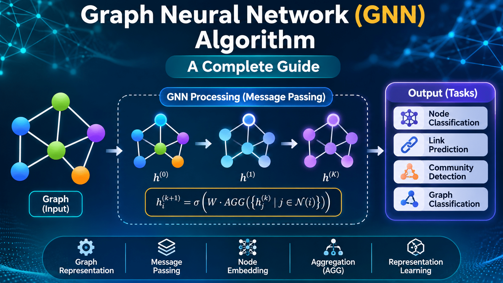
Graph Neural Network (GNN) is a family of deep learning methods designed to learn from data represented as graphs. Unlike conventional neural networks that mainly process fixed-size vectors, matrices, sequences or grids, a GNN directly models entities and the relationships connecting them. It repeatedly exchanges information between connected nodes, combines neighbouring information and learns representations that reflect both node attributes and graph structure. Graph data appears in social networks, citation networks, recommendation systems, molecular structures, transportation systems, communication networks, knowledge graphs and many other domains. This article explains the foundations of GNNs, the message-passing algorithm, mathematical formulations, a worked example, pseudocode, applications, advantages, limitations and useful research references.
What is Graph Neural Network (GNN) ?
A Graph Neural Network (GNN) is a neural network architecture that learns representations from graph-structured data. A graph consists of a set of nodes (also called vertices) and a set of edges that describe relationships between pairs of nodes. A node can represent a person, product, document, atom, web page, device or transaction. An edge can represent friendship, purchase behaviour, citation, chemical bond, communication or another meaningful relationship.
A graph is commonly represented as G = (V, E), where V is the set of nodes and E is the set of edges. Each node may have a feature vector, and each edge may optionally have attributes. The graph structure tells the model which entities can exchange information. A GNN learns by repeatedly aggregating information from the neighbourhood of each node and updating its representation.
The main concept is message passing. At each layer, a node receives messages from its neighbours, combines those messages using an aggregation function such as sum, mean, max or attention-weighted sum, and updates its hidden representation. After multiple layers, the node representation can encode information from progressively larger graph neighbourhoods. A readout or pooling operation can combine node representations when the task concerns an entire graph rather than an individual node.
For example, in a citation network, papers are represented as nodes and citation relationships as edges. A GNN can use a paper’s text-derived features together with the features of papers connected to it to classify its research topic. In a molecular graph, atoms can be nodes and chemical bonds can be edges; a graph-level representation can then support molecular property prediction.
GNN is an umbrella term rather than one single fixed architecture. Important variants include Graph Convolutional Networks (GCNs), GraphSAGE, Graph Attention Networks (GATs), graph isomorphism networks and message-passing neural networks. They share the idea of learning from graph neighbourhoods, but differ in the way they sample neighbours, calculate messages, aggregate information and update node representations.
Introduction to Graph Neural Networks (GNN)
Many real-world datasets are relational. A conventional machine learning pipeline often converts each record into an independent feature vector. This can discard useful context: two records may be closely related even when their individual attributes look similar to those of unrelated records. Graph representation preserves these connections and makes them available to the learning algorithm.
Traditional neural networks are effective for regular data arrangements. Convolutional neural networks exploit the spatial locality of images, while recurrent and transformer architectures model sequential or token relationships. Graphs, however, do not have a fixed grid layout. Nodes can have different numbers of neighbours, there is no universal left-to-right ordering, and the graph may be directed, undirected, weighted, heterogeneous or dynamic. A graph learning method therefore needs operations that work on irregular neighbourhoods and do not depend on an arbitrary ordering of nodes.
GNNs address this issue by using shared learnable functions over neighbourhoods. The same message and update functions can be applied to many nodes, which allows the model to work with graphs of different sizes. Aggregation functions such as sum and mean are permutation-invariant: rearranging the order in which a node’s neighbours are presented does not change the aggregate result. This is an important property because a neighbourhood is a set, not a naturally ordered sequence.
The modern GNN literature includes several influential directions. Kipf and Welling introduced a scalable semi-supervised Graph Convolutional Network that propagates information through a normalized adjacency matrix. GraphSAGE, proposed by Hamilton, Ying and Leskovec, learns an inductive function that samples and aggregates neighbourhood features, making it useful when unseen nodes appear. Graph Attention Networks use masked self-attention to assign different importance weights to neighbours. A broad review by Zhou and colleagues surveys GNN architectures, components and application areas.
GNN tasks are commonly grouped into three levels. Node-level tasks predict a property or label for each node, such as the topic of a paper or the risk category of an account. Edge-level tasks estimate whether a relationship exists or what type of relationship connects two nodes; link prediction is a typical example. Graph-level tasks produce a prediction for a complete graph, for example classifying a molecule or predicting a graph-level physical property.
Detailed Graph Neural Network (GNN) Algorithm
3.1 Graph representation and input data
Let the input graph be G = (V, E), containing N nodes. The node feature matrix is represented by X ∈ RN × F, where F is the number of features per node. The graph connectivity can be represented by an adjacency matrix A ∈ RN × N. For an unweighted undirected graph, Aij is 1 when nodes i and j are connected and 0 otherwise. Weighted graphs store edge weights, while directed graphs retain edge direction. Some GNN models also take an edge-feature matrix or edge attributes.
Each node i begins with an input feature vector hi(0) = xi. Features may be numerical values, encoded categories, text embeddings, image embeddings or domain-specific measurements. Feature preparation must be consistent between training and inference. Missing values, categorical variables, feature scaling and potentially sensitive attributes should be handled according to the task and data-governance requirements.
3.2 Self-loop addition
In many GCN formulations, self-loops are added so that a node can retain and use its own information in addition to receiving information from its neighbours. The adjacency matrix with self-loops is:
à = A + I
Here, I is the identity matrix. Adding I makes each node part of its own neighbourhood. Not every GNN architecture uses exactly this operation; it is a common design choice in GCN-style propagation.
3.3 Degree calculation and normalization
The degree of node i in the self-loop-augmented graph is the sum of the values in row i:
ḓi = Σj Ãij
The diagonal degree matrix is denoted by D̃, with D̃ii = ḓi. Symmetric normalization is then computed as:
 = D̃−1/2 à D̃−1/2
Normalization reduces the effect of raw node degree on message magnitude. It scales each connection according to the degrees of both its endpoint nodes. This is the standard normalized propagation used in the commonly cited two-layer GCN formulation.
3.4 Message generation
For a general message-passing GNN, each neighbour j sends a message to node i. At layer k, a message can be represented as:
mj→i(k) = φ(k)(hi(k−1), hj(k−1), eji)
Here, φ is a learnable message function, hi and hj are the current node representations, and eji is an optional edge-feature vector. The message function may be a linear transformation, a multilayer perceptron or another differentiable function. A simple model may transform the neighbour feature only; a more expressive model may combine the source node, destination node and edge attributes.
3.5 Neighbourhood aggregation
The messages arriving at node i are combined using a permutation-invariant aggregation function:
ai(k) = AGGREGATE({mj→i(k) : j ∈ N(i)})
N(i) denotes the neighbours of i. Common aggregation functions include:
- Sum: ai = Σj∈N(i) mj→i. This retains information about the total magnitude of incoming messages.
- Mean: ai = (1 / |N(i)|) Σj∈N(i) mj→i. This normalizes by the number of neighbours.
- Maximum: each feature dimension takes the maximum value among received messages.
- Attention-weighted sum: ai = Σj∈N(i) αijmj→i, where αij indicates the learned importance of neighbour j for node i.
The aggregation choice affects what structural information can be retained. For instance, mean aggregation can reduce sensitivity to neighbourhood size, while sum aggregation can preserve some count-related information. Attention allows the model to learn different weights for different neighbours.
3.6 Node representation update
After aggregation, each node updates its representation by combining the aggregated neighbourhood information with its previous representation:
hi(k) = γ(k)(hi(k−1), ai(k))
The update function γ may concatenate the old representation and aggregate, apply a linear layer, add a residual connection, and pass the result through an activation function such as ReLU. A generic example is:
hi(k) = σ(W(k)[hi(k−1) ∥ ai(k)] + b(k))
In this expression, ∥ denotes concatenation, W is a learnable weight matrix, b is a bias vector and σ is a nonlinear activation. Different architectures use different update equations.
3.7 GCN layer formulation
A common GCN layer can be written in matrix form as:
H(k) = σ(Â H(k−1) W(k))
H(0) = X. The normalized adjacency matrix  mixes information from connected nodes, W(k) learns a feature transformation, and σ introduces non-linearity. A frequently used two-layer node-classification model is:
Z = softmax(Â ReLU(Â X W(0)) W(1))
Z contains class probabilities for nodes. The number of output columns equals the number of classes. This expression is a particular GCN architecture, not a universal formula for every GNN.
3.8 Readout and prediction
After K message-passing layers, node embeddings contain information aggregated from up to K graph hops, subject to the architecture and graph connectivity. For node classification, a classifier can map each final node representation to class scores:
ŷi = softmax(Wc hi(K) + bc)
For graph-level prediction, the model combines the node representations using a readout function, for example:
hG = READOUT({hi(K) : i ∈ V})
READOUT may use sum, mean, maximum, attention pooling or a more structured pooling operation. The graph embedding hG is then passed to a classifier or regression head. Edge prediction commonly uses a scoring function over the embeddings of two candidate nodes, optionally with edge features.
3.9 Loss function and model training
For supervised node classification with labelled training nodes L, cross-entropy loss is commonly used:
ℒ = − Σi∈L Σc=1C yic log Zic
Here, yic is the one-hot target label and Zic is the predicted probability for class c. The model parameters are optimized using gradient-based methods such as Adam or stochastic gradient descent. Regularization, weight decay, dropout and early stopping may be used to control overfitting. For regression, a loss such as mean squared error may be appropriate; link prediction often uses binary cross-entropy or ranking objectives.
3.10 Model evaluation and inference
After training, evaluate the model on validation and test data that are separated according to the intended deployment setting. Accuracy, precision, recall, F1-score and area under the ROC curve may be appropriate for classification, but the metric should match class balance and application cost. Regression tasks require measures such as MAE or RMSE. For link prediction, ranking metrics such as mean reciprocal rank or Hits@K may be used. Avoid data leakage: for example, do not allow test labels or future graph edges to influence the training representation when the real-world task requires predicting them.
Step-by-Step Explanation of the GNN
Step 1 – Define the graph learning problem. First, identify what each entity represents and what relationships connect them. Decide whether the objective is node classification, edge prediction, graph classification or regression. This decision determines the required input, output layer, training labels and evaluation strategy. For example, if the objective is to identify the topic of research papers, each paper becomes a node, citation links become edges and the target is a node-level class.
Step 2 – Construct the graph and prepare features. Convert the source data into a graph containing nodes and edges. Build a feature vector for each node using available attributes such as numerical measurements, categorical encodings or learned text representations. If relationships have meaningful properties, preserve them as edge features. Check the graph for duplicate edges, invalid identifiers, missing attributes and incorrect direction. In temporal problems, record timestamps so that future information does not leak into past predictions.
Step 3 – Initialize node representations. Each node receives an initial embedding based on its input feature vector. In a simple model, the initial hidden state is identical to the prepared feature vector. In more complex models, an embedding layer projects raw input into a hidden dimension suitable for message passing. The same learnable transformation is typically shared across nodes, so the network can process different graph regions using a consistent representation space.
Step 4 – Prepare graph connectivity for propagation. The model uses the adjacency structure to identify which nodes can exchange messages. In a GCN, self-loops are often added and the adjacency matrix is symmetrically normalized. In GraphSAGE, a fixed or sampled number of neighbours may be selected at each layer to control computation. In a GAT, attention coefficients are calculated over a node’s neighbourhood. The exact preparation therefore depends on the chosen GNN variant.
Step 5 – Generate messages from neighbouring nodes. During each layer, a node gathers information from its connected neighbours. A message function transforms the neighbour representation and may also incorporate the current node representation and edge attributes. This operation allows the network to learn which feature information should be passed across each relationship. The message function is shared across many graph connections, helping the model learn a common relational pattern instead of building a separate network for every node.
Step 6 – Aggregate the messages. The received messages are combined into a single neighbourhood summary. A sum, mean or maximum operation can be used, or an attention mechanism can assign a learned coefficient to each neighbour before combining the messages. The aggregation must not depend on an arbitrary ordering of neighbours. This stage is important because real-world nodes may have two neighbours, hundreds of neighbours or no neighbours at all.
Step 7 – Update the node embedding. The aggregated summary is combined with the node’s previous representation. A learnable update function, commonly built from linear layers and nonlinear activation, creates a new embedding. The network thus balances information from the node itself and information received from its local graph context. Optional residual connections, normalization layers and dropout can improve optimization and generalization.
Step 8 – Repeat message passing across layers. The model repeats message generation, aggregation and updating for the selected number of layers. A one-layer GNN mainly captures immediate neighbours. A two-layer GNN can incorporate information from nodes two edges away, and additional layers expand the receptive field further. However, using more layers is not always better: very deep message passing can make node representations too similar, a problem commonly called over-smoothing. The number of layers should be selected through validation and domain knowledge.
Step 9 – Produce task-specific outputs. The final node embeddings are passed to a prediction head for node-level tasks. If the target is an entire graph, a readout function combines the node embeddings into a graph representation. For edge prediction, the model scores pairs of node embeddings. A softmax output is often used for multi-class classification, while sigmoid outputs may be used for binary or multi-label predictions.
Step 10 – Calculate loss and optimize parameters. Compare model predictions with the ground-truth labels available for the training split. Calculate an appropriate loss, backpropagate its gradients and update the trainable parameters using an optimizer. Repeat this process across mini-batches or training epochs until the validation metric stops improving or another stopping condition is reached. A separate test split should be used for final reporting rather than for repeated hyperparameter decisions.
Step 11 – Evaluate and deploy carefully. Assess the model using metrics suited to the task, inspect errors across important subgroups and compare against simple baselines. At deployment, ensure that new nodes and edges are represented in a way consistent with training. Inductive approaches can generate embeddings for unseen nodes from their features and neighbourhoods, while some transductive approaches assume a largely fixed graph. Monitor changes in graph structure and feature distributions because relationships can evolve over time.
Example of How a Graph Neural Network Works
Example: Research paper topic classification
Consider a small citation network containing four research papers: Paper A, Paper B, Paper C and Paper D. Each paper is a node. A directed edge from Paper B to Paper A means that B cites A. For a simplified illustration, suppose the graph relationships used for neighbourhood aggregation connect A with B and C, while B and C are also connected to D. Each paper has two input features derived from its content: the first feature indicates the strength of a computing-related term representation, and the second indicates the strength of a biology-related term representation. These values are illustrative, not empirical measurements.
| Node | Initial feature vector | Neighbourhood (illustrative) | Known training class |
|---|---|---|---|
| Paper A | [1.0, 0.0] | B, C | Computing |
| Paper B | [0.8, 0.2] | A, D | Computing |
| Paper C | [0.2, 0.8] | A, D | Biology |
| Paper D | [0.1, 0.9] | B, C | Biology |
Step 1: Encode the graph. The four papers are represented as nodes and their citation relationships as edges. The input feature matrix is:
X = [[1.0, 0.0], [0.8, 0.2], [0.2, 0.8], [0.1, 0.9]]
The adjacency structure stores the connectivity. For this simplified explanation, we use an undirected neighbourhood view so the aggregation arithmetic is easy to follow. A production citation model may retain edge direction or use separate incoming and outgoing message functions.
Step 2: Aggregate the neighbour features for Paper A. A mean aggregator combines the vectors of B and C:
mean(B, C) = ([0.8, 0.2] + [0.2, 0.8]) / 2 = [0.5, 0.5]
This summary contains information from the local neighbourhood. Paper A’s own vector is [1.0, 0.0]. A simple illustrative update can concatenate its own vector with the mean neighbourhood vector:
hA(1) = [1.0, 0.0 ∥ 0.5, 0.5] = [1.0, 0.0, 0.5, 0.5]
A real GNN would normally apply learnable weights and a nonlinear activation to this concatenated representation. The concatenation here is shown only to make the information flow visible.
Step 3: Perform aggregation for other nodes. Paper B receives information from A and D. Its mean neighbour vector is ([1.0, 0.0] + [0.1, 0.9]) / 2 = [0.55, 0.45]. Paper C receives information from A and D, giving the same mean vector in this deliberately small example. Paper D receives information from B and C, producing ([0.8, 0.2] + [0.2, 0.8]) / 2 = [0.5, 0.5]. Each node therefore receives a different combination of its own feature information and its neighbours’ feature information.
Step 4: Transform and update. The network applies shared learnable weight matrices to the combined representations and uses an activation function such as ReLU. During training, the weights are adjusted so that representations become useful for separating the target classes. If more message-passing layers are used, the nodes can incorporate information from a wider part of the citation network.
Step 5: Predict the class. A classification layer converts the final embedding of each paper into class scores. A softmax function turns those scores into probabilities. The largest probability is selected as the predicted class. For an unseen paper, its content features and its graph connections can be used to generate a representation and estimate its topic, provided the trained model supports the intended inductive or transductive setting.
This example shows why a GNN is different from a model that classifies every paper independently. The prediction can use both the paper’s own content and information from connected papers. However, neighbour similarity is not guaranteed: citation links may cross research areas, and graph relationships may be noisy. The training objective and validation process must teach the model how to use these relationships appropriately.
The following process diagram summarizes a typical message-passing GNN pipeline, from graph input to prediction and model optimization.
Nodes, edges, node / edge features
Adjacency, self-loops, normalization / sampling
Transform neighbour information
Sum, mean, max or attention
Combine self and neighbourhood
Learn multi-hop node representations
Node or graph representation
Class, link score or value
Backpropagation · parameter update · evaluation
Figure: General message-passing workflow of a Graph Neural Network. Specific architectures may change the graph preparation, message, aggregation, update and readout modules.
Pseudocode for Graph Neural Network (GNN) Algorithm
The following generic pseudocode describes supervised node classification using a message-passing GNN. It is architecture-neutral: the message, aggregation and update functions can be implemented as a GCN, GraphSAGE, GAT or another suitable model.
Algorithm: Message-Passing Graph Neural Network

Input:
    G = (V, E)                 // Input graph
    X                          // Node feature matrix
    Y                          // Labels for training nodes
    L_train                    // Training node indices
    K                          // Number of message-passing layers
    epochs                     // Maximum training epochs
    learning_rate              // Optimizer learning rate

Output:
    Trained parameters θ
    Predicted labels or scores

1.  Initialize trainable parameters θ
2.  Set h_i(0) = x_i for every node i in V
3.  Prepare graph connectivity (add self-loops / normalize
    or configure neighbourhood sampling as required)

4.  For epoch = 1 to epochs:
5.      For each GNN layer k = 1 to K:
6.          For each node i in V:
7.              messages = empty collection
8.              For each neighbour j in N(i):
9.                  m_ji = MESSAGE(h_i(k-1), h_j(k-1), e_ji; θ_k)
10.                 Add m_ji to messages
11.             end for
12.             a_i = AGGREGATE(messages)
13.             h_i(k) = UPDATE(h_i(k-1), a_i; θ_k)
14.         end for
15.     end for

16.     For each training node i in L_train:
17.         scores_i = PREDICT(h_i(K); θ_head)
18.     end for

19.     loss = LOSS(scores, Y on L_train)
20.     Compute gradients of loss with respect to θ
21.     Update θ using the selected optimizer
22.     Evaluate on validation data
23.     Apply early stopping when the stopping criterion is met
24. end for

25. Run the trained model on the required graph
26. Return predicted scores / labels and trained parameters
In a practical implementation, iterating over every node and every edge in nested loops is usually replaced by vectorized tensor operations, sparse matrix multiplication or framework-specific message-passing routines. Large graphs may use neighbour sampling, graph partitioning, mini-batch training or distributed computation. The pseudocode expresses the conceptual algorithm rather than an optimized implementation.
Advantages and Disadvantages of Graph Neural Network (GNN)
Advantages
- Uses relationships explicitly: GNNs learn from both node attributes and graph connectivity, which is valuable when interactions carry predictive information.
- Flexible graph structures: Message-passing architectures can handle irregular neighbourhood sizes and graphs without a fixed grid arrangement.
- Multiple prediction levels: GNNs support node classification, link prediction, graph classification and regression through suitable output and readout layers.
- Shared learnable operations: A common message and update function is applied across graph nodes and edges, supporting parameter sharing.
- Combines multiple data types: Node and edge attributes can represent numerical, categorical, textual, molecular or other domain features.
- Context-aware representations: Multiple layers allow a node representation to incorporate information from multi-hop neighbourhoods.
- Inductive learning is possible: Architectures such as GraphSAGE learn aggregation functions that can generate representations for unseen nodes when their features and neighbourhood information are available.
Disadvantages and challenges
- Computational cost: Message passing can be expensive for large or dense graphs, especially when many layers or large neighbourhoods are involved.
- Dependence on graph quality: Missing, noisy or biased edges can distort the information exchanged between nodes. A poorly constructed graph can reduce prediction quality.
- Over-smoothing: With many propagation layers, node representations can become increasingly similar, making it harder to distinguish nodes.
- Over-squashing: Information from a large or expanding receptive field may be compressed into fixed-size vectors, limiting how much distant information can be retained.
- Heterophily challenge: In some networks, connected nodes have different labels or attributes. Methods relying heavily on neighbour similarity may not perform well unless designed for such settings.
- Data leakage risks: Incorrect graph splitting can expose validation or test information during training, producing overly optimistic evaluation results.
- Interpretability: It can be difficult to explain exactly which neighbours, edges and features caused a prediction, even when attention weights are available.
- Dynamic graph maintenance: Frequently changing nodes and relationships require suitable updates, temporal modelling and monitoring procedures.
- Class imbalance and fairness: Rare classes, uneven node degree and biased connectivity can lead to unequal performance across groups.
These limitations do not make GNNs unsuitable; they indicate that graph construction, model selection, splitting strategy, scaling and evaluation are essential parts of a reliable graph-learning project. A strong baseline, such as a feature-only model or a simple graph method, should be included to test whether graph information actually adds value.
Applications of Graph Neural Network (GNN) Algorithm
Social network analysis
In social networks, users are represented as nodes and relationships or interactions are represented as edges. GNNs can support community-related prediction, user classification, recommendation, link prediction and suspicious account detection. The model can combine profile attributes with interaction patterns, subject to privacy, consent and fairness requirements.
Recommendation systems and e-commerce
Products, customers, sessions and transactions can be represented in a heterogeneous graph. Edges may represent views, clicks, purchases, reviews or co-purchase relationships. A GNN can learn user and item embeddings from this relational structure and use them for candidate ranking or recommendation. Care is required to prevent future interactions from leaking into training and to evaluate recommendation quality with realistic time-based splits.
Drug discovery and molecular property prediction
A molecule can be represented as a graph in which atoms are nodes and chemical bonds are edges. Node features may include atom type, valence or formal charge, while edge features may describe bond type. Message-passing neural networks can learn molecular representations useful for predicting selected chemical or biological properties. Experimental validation remains essential before using predictions for scientific or clinical decisions.
Healthcare and biomedical networks
Biomedical graphs can connect patients, diseases, drugs, genes, proteins and clinical concepts. GNNs may be studied for patient similarity, drug-disease association, protein interaction analysis and risk prediction. Clinical use requires careful validation, patient privacy protection, attention to population bias and assessment by qualified domain experts.
Knowledge graphs and natural language processing
Knowledge graphs store entities and their relationships, such as person–organization, drug–condition or concept–definition links. GNNs can learn entity representations for link prediction, relation classification and knowledge graph completion. In NLP, graphs can represent syntactic dependency trees, document citations or entity relations, allowing a neural model to combine text representations with explicit structure.
Cybersecurity and fraud detection
Devices, IP addresses, accounts, transactions and network sessions can form security graphs. GNNs can help identify suspicious relationships, detect coordinated behaviour, classify potentially malicious nodes and rank risky transaction links. Because attackers can manipulate graph structure and feature values, robustness testing and continuously updated threat models are important.
Transportation and traffic prediction
Road intersections or road segments can be represented as nodes, with roads or traffic connections as edges. A graph model can combine sensor readings with network topology to estimate traffic conditions or predict congestion. Temporal GNN architectures combine graph message passing with time-series components to model both spatial relationships and changes over time.
Communication networks and IoT
In communication and Internet of Things systems, sensors, routers, gateways and devices can be graph nodes, while communication links form edges. GNNs can be investigated for traffic forecasting, fault detection, resource allocation and network anomaly detection. Deployment must consider changing topology, limited device resources, latency requirements and the cost of collecting graph data.
Citation networks and academic research
Research papers can be represented as nodes and citation links as edges. Node attributes may include title or abstract embeddings, author information and publication metadata. GNNs can support paper topic classification, citation-link prediction, document recommendation and scholarly knowledge discovery. Train/test design should respect publication time when the objective is to predict future citations or emerging topics.
Conclusion
Graph Neural Networks provide a general deep learning framework for learning from graph-structured data. Their central mechanism is message passing: nodes exchange information with their neighbours, aggregate the received messages and update their hidden representations. Repeating this process enables a node to incorporate information from increasingly broad graph neighbourhoods. A readout layer can further transform node representations into graph-level predictions.
The GNN family includes GCN, GraphSAGE, GAT and many other architectures. The appropriate method depends on graph size, feature availability, graph direction, homophily or heterophily, dynamic behaviour, task type and computational constraints. Mathematical formulations such as normalized graph convolution provide a clear starting point, while attention, sampling and edge-aware message functions offer alternative design choices.
GNNs have broad potential in social networks, recommendation, chemistry, healthcare research, cybersecurity, transportation, IoT and knowledge graphs. However, their effectiveness depends on graph quality, leakage-free evaluation, scalable implementation and careful attention to bias and privacy. Researchers should compare a proposed GNN with meaningful baselines, report suitable metrics and document the graph construction and data-splitting strategy. With these practices, GNNs can provide a useful approach to modelling complex relationships that are difficult to represent using independent feature vectors alone.
Frequently Asked Questions (FAQs)
FAQ 1. What is a Graph Neural Network (GNN) in simple terms?
A Graph Neural Network is a deep learning model that learns from objects and the relationships between them. Each object is a node, each relationship is an edge, and the model shares information between connected nodes to build context-aware representations.
FAQ 2. What is the main working principle of a GNN?
The main principle is message passing. A node receives information from its neighbours, aggregates the messages using an operation such as sum, mean, max or attention, and updates its representation. This process is repeated over multiple layers.
FAQ 3. What is the difference between GCN, GraphSAGE and GAT?
GCN commonly uses normalized adjacency-based feature propagation. GraphSAGE samples and aggregates neighbourhood features and is designed to support inductive representation learning. GAT uses attention coefficients to learn different importance weights for neighbours. All are GNN variants, but their aggregation and propagation mechanisms differ.
FAQ 4. What are the main applications of GNN algorithms?
Common research and application areas include social network analysis, recommendation systems, molecular property prediction, biomedical networks, knowledge graphs, cybersecurity, traffic forecasting, IoT and citation-network analysis. The model must be selected and validated for the specific domain and task.
FAQ 5. Can a GNN work with large graphs?
Yes, but large graphs require careful engineering. Neighbour sampling, mini-batch training, sparse matrix operations, graph partitioning and distributed processing can reduce memory and computation demands. Frameworks such as PyTorch Geometric provide tools for implementing message-passing layers and graph sampling workflows.
FAQ 6. What are the main limitations of Graph Neural Networks?
Important limitations include computational cost, sensitivity to graph quality, over-smoothing in deep models, over-squashing of distant information, difficulty with some heterophilous graphs, interpretability challenges and data leakage risks. Model evaluation should include appropriate baselines and realistic graph splits.
References
- Zhou, J., Cui, G., Hu, S., Zhang, Z., Yang, C., Liu, Z., Wang, L., Li, C., & Sun, M. (2020). “Graph Neural Networks: A Review of Methods and Applications.” AI Open, 1, 57–81. https://doi.org/10.1016/j.aiopen.2021.01.001
- Kipf, T. N., & Welling, M. (2017). “Semi-Supervised Classification with Graph Convolutional Networks.” International Conference on Learning Representations (ICLR). https://arxiv.org/abs/1609.02907
- Hamilton, W., Ying, Z., & Leskovec, J. (2017). “Inductive Representation Learning on Large Graphs.” Advances in Neural Information Processing Systems (NeurIPS), 30. NeurIPS paper page
- Veličković, P., Cucurull, G., Casanova, A., Romero, A., Liò, P., & Bengio, Y. (2018). “Graph Attention Networks.” International Conference on Learning Representations (ICLR). OpenReview paper page
- PyTorch Geometric Team. “Creating Message Passing Networks.” PyTorch Geometric Documentation. Official documentation
Further learning: Explore the PyTorch Geometric documentation for practical GNN implementation, the original GCN paper for the normalized convolution formulation, and the GraphSAGE paper for inductive neighbourhood aggregation.