What is the Linear Regression Algorithm?
Linear regression is a supervised learning algorithm that models the relationship between one or more input variables (features) and a continuous output variable (target) by fitting a straight line (or hyperplane) to observed data. In its simplest form—simple linear regression—we assume the target y changes linearly with a single feature x. The model is:

Where y^ is the predicted target, β0 is the intercept, and β1 is the slope (also called the coefficient or weight). For multiple features x1,x2,…,xp , we use multiple linear regression:

Linear regression is foundational in statistics and machine learning because it’s easy to interpret, efficient to train, and surprisingly powerful for many real-world problems like forecasting sales, estimating house prices, or modeling physical processes.
Introduction to the Linear Regression Algorithm
At its heart, linear regression is about finding the best-fitting line through data. “Best” is defined by an objective function—commonly the Sum of Squared Errors (SSE) or the Mean Squared Error (MSE)—which measures how far predictions y^i are from the true values yi . We want coefficients β that minimize:

There are two standard ways to find these coefficients:
- Closed-form solution (Normal Equation): Solve an algebraic formula that directly gives the optimal coefficients—fast for small to moderate feature sets.
- Iterative optimization (Gradient Descent): Start with random coefficients and repeatedly move them in the direction that reduces error—scales well to very large datasets and feature spaces.
Beyond fitting, linear regression assumes:
- Linearity: The relationship between features and the target is additive and linear in parameters.
- Independence of errors: Residuals (errors) are independent across observations.
- Homoscedasticity: Residuals have constant variance.
- Normality of errors (for inference): Residuals are normally distributed (useful when building confidence intervals and hypothesis tests).
- Low multicollinearity: Features are not highly correlated with each other; otherwise, estimates become unstable.
In practice, we validate these assumptions with residual plots, correlation checks, and goodness-of-fit metrics. When assumptions are violated, we might transform variables, engineer features, or switch to more robust or nonlinear models.
The Linear Regression Algorithm
This section lays out the full algorithmic flow—from raw data to trained model—covering both the Normal Equation and Gradient Descent approaches.
Notation and Setup
- We have n observations.
- In multiple regression with p features, define:
- X∈Rn×(p+1) as the design matrix, where the first column is all ones for the intercept, and the remaining ppp columns are features.
- y∈Rn as the vector of targets.
- β∈R(p+1) as the vector of coefficients [β0,β1,…,βp]T.
- Prediction for all samples: y^=Xβ.
- Residuals: r=y−y^=y−Xβ.
Objective Function (Least Squares)

The factor 1/ 2n is standard in optimization to simplify gradients.
Normal Equation (Closed Form)
Set the gradient of J(β) to zero and solve:

If XTX is invertible,
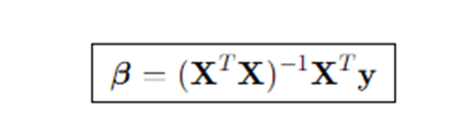
This yields the unique least-squares solution.
Note on Regularization: To handle multicollinearity or improve generalization, we can use Ridge Regression (L2 penalty), modifying the normal equation to:

Where, λ≥0 controls shrinkage. (Lasso uses an L1 penalty and is usually solved iteratively.)
Batch Gradient Descent
When p is large or n is massive, iterative methods are preferred.
Initialize: Choose β(0) (often zeros).
Repeat for t=0,1,2,… until convergence:

Where, α is the learning rate.
Variants:
- Stochastic Gradient Descent (SGD): Update using one sample at a time—cheap, noisy updates, good for streaming/big data.
- Mini-batch Gradient Descent: Update with small batches (e.g., 32–1024 samples)—balances stability and efficiency.
Convergence Criteria: Stop when parameter changes or objective reduction falls below a small threshold, or after a max number of iterations.
Feature Scaling and Intercept Handling
- Scaling/Standardizing: For gradient descent, scale features so they have similar magnitudes (e.g., zero mean, unit variance). This dramatically improves convergence.
- Intercept: Include a column of ones in X. If you standardize, compute the intercept on the original scale or center y accordingly.
Model Evaluation Metrics
After training, use these metrics:
- R-squared R2=1−∑(yi−yˉ)2∑(yi−y^i)2.
- Adjusted R2: penalizes adding many features.
- MSE / RMSE: average squared error and its square root.
- MAE: mean absolute error (more robust to outliers).
- Residual Analysis: plot residuals vs. fitted values to check patterns (should look random if assumptions hold).
Step-by-Step Explanation of the Algorithm
Step 1: Define the problem and collect data. Begin by clearly articulating the target you want to predict (e.g., house price) and the features you believe explain it (e.g., size, bedrooms, locality). Gather a dataset with sufficient samples and ensure the target is continuous. Split the data into training and test sets to evaluate generalization; optionally keep a validation set or use cross-validation for model selection.
Step 2: Inspect, clean, and preprocess. Explore distributions, missing values, and outliers. Clean the data by handling missingness (deletion, mean/median imputation, model-based imputation), fixing data types, and addressing obvious errors. Consider log transforms for skewed variables and encode categorical variables (one-hot encoding) if you plan to use linear regression with categorical inputs.
Step 3: Engineer features and check multicollinearity. Create derived features that better capture relationships (e.g., price per square foot, interaction terms such as x1x2, polynomial terms like x2). Evaluate correlations and compute Variance Inflation Factor (VIF) to spot multicollinearity. If VIFs are high, drop or combine collinear features, or use Ridge/Lasso to stabilize estimates.
Step 4: Choose an estimation method. If the number of features is modest and the dataset fits in memory, use the normal equation for a fast, exact solution. If the dataset is huge—or you expect to stream data—choose gradient descent (batch, mini-batch, or SGD). For gradient descent, standardize features and pick a sensible learning rate; consider using learning-rate schedules.
Step 5: Fit the model. For the normal equation, construct the design matrix X with a leading column of ones and compute β=(XTX)−1XTy. For gradient descent, iteratively update β in the negative gradient direction until convergence, monitoring loss reduction and validation performance to avoid overfitting.
Step 6: Diagnose the fit. Compute R2, RMSE, and MAE on both training and test sets. Inspect residual plots to confirm that residuals look unstructured and have constant variance; funnel shapes suggest heteroscedasticity, and curves suggest nonlinearity. A Q–Q plot helps assess normality. Use leverage and Cook’s distance to detect influential points.
Step 7: Refine the model. If diagnostics raise concerns, revisit feature engineering. Nonlinearity can be handled by polynomial terms or splines; heteroscedasticity may improve with log transforms of the target or weighted least squares; multicollinearity may require dimensionality reduction (PCA) or regularization (Ridge/Lasso/Elastic Net). Iterate until performance is acceptable and assumptions are reasonably satisfied.
Step 8: Interpret and communicate. Translate coefficients into domain language. For example, a slope of 2500 for “square feet” means “each additional square foot increases price by ₹2,500 on average, holding other features constant.” Provide confidence intervals and discuss limitations and practical implications.
Step 9: Deploy and monitor. Once validated, deploy the model into production. Monitor prediction errors over time; if data drift occurs (e.g., market changes), retrain or recalibrate the model. Keep a reproducible training pipeline with versioned data and code.
Example: How Linear Regression Works
Consider a simple dataset that pairs a single feature x with a target y. Suppose we have five observations:
| i | xi | yi |
| 1 | 1.0 | 2.0 |
| 2 | 2.0 | 2.8 |
| 3 | 3.0 | 3.6 |
| 4 | 4.0 | 4.5 |
| 5 | 5.0 | 5.1 |
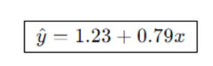
We’ll fit a simple linear regression y^=β0+β1x using the closed-form formulas for slope and intercept (equivalent to the normal equation for one feature).
First compute the means:

Compute the numerator and denominator for the slope:
Tabulate terms:
| i | xi−xˉ | yi−yˉ | Product (xi−xˉ)(yi−yˉ) | (xi−xˉ)2 |
| 1 | -2 | -1.6 | 3.2 | 4 |
| 2 | -1 | -0.8 | 0.8 | 1 |
| 3 | 0 | 0.0 | 0.0 | 0 |
| 4 | 1 | 0.9 | 0.9 | 1 |
| 5 | 2 | 1.5 | 3.0 | 4 |
So

Slope and intercept:

Thus the fitted line is:
Predictions for each x are close to the observed y. The residual for, say,


Advantages and Disadvantages of the Linear Regression
Advantages
- Simplicity and Interpretability: Coefficients have direct, human-readable meanings (change in y per unit change in xj, holding others constant). Decision-makers love it.
- Efficiency: Training is computationally cheap; the closed-form solution is fast for modest p, and gradient descent scales to very large datasets.
- Baseline Quality: It’s an excellent baseline; any more complex model should beat it on validation before being adopted.
- Analytical Toolkit: Comes with a rich statistical ecosystem—confidence intervals, hypothesis tests, ANOVA decompositions, and diagnostics that guide improvements.
- Extensibility: Easy to add regularization (Ridge, Lasso), interactions, and polynomial features to capture moderate nonlinearity.
Disadvantages
- Linearity Assumption: If the true relationship is nonlinear or strongly interactive, a straight line will be biased, even with abundant data.
- Sensitivity to Outliers: Squaring errors gives extreme weight to outliers; a few bad points can dominate the fit.
- Multicollinearity: Highly correlated features inflate variance of estimates, making coefficients unstable and hard to interpret.
- Heteroscedasticity and Autocorrelation: Violations of constant variance or independence degrade inference and can mislead standard errors and tests.
- Extrapolation Risk: Predictions outside the observed feature range are often unreliable; the straight line continues forever, but reality doesn’t.
- Limited Expressiveness: Without feature engineering, linear regression cannot model complex patterns that tree-based methods or neural nets capture natively.
Applications of Linear Regression
- Economics & Finance: Forecasting sales, revenue, or demand from price and marketing spend; estimating beta in CAPM; modeling credit risk drivers in scorecards (with suitable transforms).
- Real Estate: Predicting house prices from size, location, age, and amenities; rent estimation for property management.
- Healthcare & Epidemiology: Modeling clinical measurements (e.g., blood pressure vs. age and BMI); estimating dose-response relationships; health cost prediction.
- Manufacturing & Quality Control: Relating process parameters to yield or defect rates; cost modeling; predictive maintenance features vs. failure times (when treated appropriately).
- Marketing & Customer Analytics: Understanding how impressions, clicks, and promotions affect conversions and lifetime value; incrementality analyses (with caveats).
- Energy & Environment: Forecasting electricity consumption from weather variables and time-of-day; modeling emissions as a function of process controls.
- Transportation & Logistics: Estimating delivery times from distance, traffic, and stops; fuel consumption vs. load and speed.
- Sports Analytics: Predicting performance metrics from training loads, player characteristics, and environmental factors.
- Science & Engineering: Calibration curves, physical law approximations (e.g., linearized relationships), and experiment analysis.
- Education & Social Sciences: Modeling test scores from study hours, instructional strategies, and demographics (with care regarding causality and fairness).
Conclusion
Linear regression endures because it strikes a rare balance: transparent, fast, and useful. With a few lines of algebra, it turns raw data into a model you can explain to a nontechnical audience. Although its assumptions are idealizations, the algorithm remains robust when paired with sound practice—thoughtful preprocessing, feature engineering, careful diagnostics, and, when needed, regularization to control variance. When the relationship is approximately linear or when interpretability is paramount, linear regression should be your first stop. Even in complex pipelines, it’s a gold-standard baseline and a powerful tool for quick insights and dependable forecasts. The key to success is discipline: split your data, validate assumptions, interpret coefficients responsibly, and monitor performance after deployment. If diagnostics suggest nonlinearity, heteroscedasticity, or multicollinearity, remember that linear regression has an extended family (Ridge, Lasso, Elastic Net, polynomial features, interactions, weighted least squares) ready to help. And when the problem demands nonlinear expressiveness, let linear regression guide you as a benchmark before scaling up to trees, ensembles, or neural networks.
Frequently Asked Questions (FAQs)
How do I know if linear regression is appropriate for my problem?
Check a scatter plot of y versus each feature and inspect residual plots after a preliminary fit. If relationships look roughly linear, residuals show no clear pattern, and performance is reasonable, linear regression is appropriate. If not, consider feature transforms, interaction terms, or nonlinear models.
What’s the difference between OLS, Ridge, and Lasso?
OLS (ordinary least squares) minimizes squared errors with no penalty. Ridge adds an L2 penalty on coefficients, shrinking them toward zero to reduce variance and handle multicollinearity. Lasso adds an L1 penalty, which can force some coefficients to be exactly zero, performing variable selection as well as shrinkage.
Why is my gradient descent not converging?
Often because features are on very different scales or the learning rate α is too large. Standardize features (zero mean, unit variance), lower α, and monitor the training loss over iterations. Mini-batch or momentum methods can also stabilize training.
How should I handle categorical variables in linear regression?
Use one-hot encoding (create binary dummy variables for each category), leaving out one category per feature as a reference level to avoid the dummy variable trap. Consider high-cardinality encodings (e.g., target encoding) carefully to avoid leakage; cross-validation helps.
Can linear regression establish causality?
No—linear regression establishes association, not causation. To infer causality, you need a research design (randomized experiments, natural experiments, instrumental variables, or careful observational methods) that addresses confounding, selection bias, and endogeneity.