Gradient Boosting is one of those rare ideas in machine learning that’s both simple at its core and remarkably powerful in practice. From credit scoring and click-through prediction to anomaly detection and forecasting, gradient boosting models (GBMs) and their popular implementations (XGBoost, LightGBM, CatBoost, scikit-learn’s GradientBoosting* classes) routinely sit near the top of leaderboards and production stacks. This guide walks you through the concept, the math, the step-by-step workflow, and practical tips—ending with advantages, limitations, applications, and FAQs.

What Is the Gradient Boosting Algorithm?

Gradient Boosting is an ensemble method that builds a strong predictor by sequentially adding weak learners (most commonly decision trees) to correct the errors of the current ensemble. Each new learner is trained to fit the negative gradient of a specified loss function with respect to the current model’s predictions—hence the name gradient boosting. In plainer words: start with a simple model; look at where it’s wrong; fit a new model to those mistakes; add it in; repeat. The procedure is generic: pick a loss (for regression, classification, ranking, quantile, etc.), and gradient boosting will push the model in the direction that most reduces that loss.

Key ideas:

• Additive modeling: build

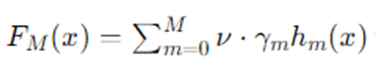
Where, h_m​ are weak learners (trees), γ_m are learner weights, and ν is a shrinkage (learning rate).

• Functional gradient descent: instead of optimizing parameters directly, we iteratively step in function space along the negative gradient of the loss.

Introduction to Gradient Boosting

2.1 Boosting vs. Bagging

• Bagging (e.g., Random Forests) trains many learners independently on bootstrapped samples and averages results to reduce variance.
• Boosting trains learners sequentially; each learner focuses on correcting the predecessor’s errors, primarily reducing bias (while regularization keeps variance in check).

2.2 Why Trees as Base Learners?

Decision trees are:

• Flexible and nonlinear, capturing interactions without manual feature engineering.
• Fast to fit and evaluate in shallow depth.
• Interpretable at the leaf level (partial dependence, SHAP, etc.).

2.3 Choice of Loss

The algorithm is agnostic to loss:

• Regression: squared error L(y,F)=1/2(y−F)² or absolute error for robustness.
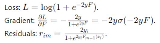
• Binary classification: logistic loss L(y,F)=log⁡ ⁣(1+e^−2yF) with y∈{−1,+1}.
• Multiclass: softmax cross-entropy.
• Quantile / Huber: for robust regression.
• Ranking: pairwise or listwise losses.

The Detailed Gradient Boosting Algorithm

Consider data {(xi​,yi​)}_i=1^N​, a differentiable loss L(y,F(x)), and a function F(x) built additively from weak learners.

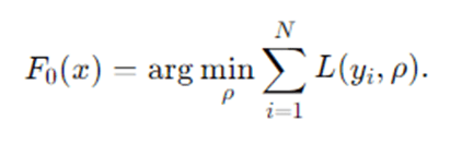
1. Initialize the model

Choose an initial constant predictor that minimizes the loss:

Examples:

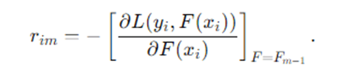
Compute pseudo-residuals (negative gradients) for each sample:

Squared error → F₀=mean(y).

Logistic loss → F₀=1/2 log (p/ 1−p) ​ is the empirical positive rate.

For m=1,2,…,M (number of boosting rounds):

Intuition: where the current model is wrong and by how much.

2. Fit a weak learner hm(x) (e.g., a regression tree) to the training set {(xi,rim)} by least squares.
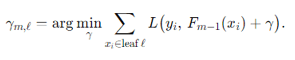
3. Compute the optimal step size (line search) for each leaf ℓ of the tree or globally:

For squared error, this reduces to averaging residuals in each leaf.

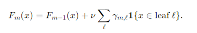
2. Update the model with learning rate ν∈[0,1]:

Return final model FM(x).

Specialization to Common Losses

• Squared error (regression)

Residuals: r_im=y_i−F_m−1(xi)

Leaf value: γ_m,ℓ=mean_xi∈ℓ(r_im)

• Logistic loss (binary, y∈{−1,+1} )

Often simplified via probability p_i=σ(2F_m−1(x_i)) and using Newton updates in some implementations.

• Huber / Quantile

Provide robustness to outliers by clipping or asymmetric penalization; residuals become piecewise expressions.

Pseudocode

Input: Data {(x_i, y_i)}_{i=1..N}, loss L(y, F), base learner Tree(),

       learning rate ν, rounds M

F0(x) = argmin_ρ Σ_i L(y_i, ρ)

for m = 1..M:

    r_i = – [∂L(y_i, F(x_i)) / ∂F(x_i)] evaluated at F = F_{m-1}

    h_m = Tree().fit(X, r)   # regression tree on pseudo-residuals

    For each leaf ℓ in h_m:

        γ_{m,ℓ} = argmin_γ Σ_{i in ℓ} L(y_i, F_{m-1}(x_i) + γ)

    F_m(x) = F_{m-1}(x) + ν * Σ_ℓ γ_{m,ℓ} 1{x ∈ leaf ℓ}

Return F_M

Step-by-Step Explanation

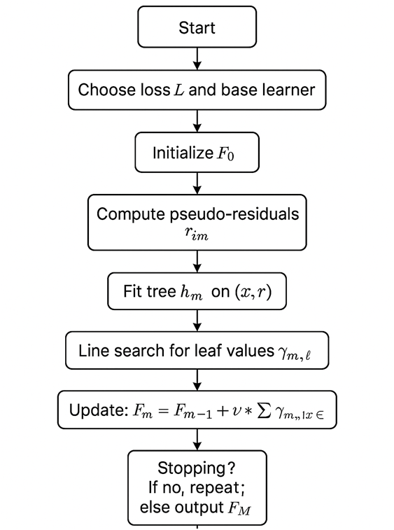
Gradient Boosting begins by picking a simple starting prediction—for regression, this could be the average target; for binary classification, a log-odds based on the class balance. Next, it examines how wrong this starting model is on each training example. These “errors” aren’t just raw differences; they are the negative gradients of the chosen loss with respect to the model’s output, which tells us the best local direction to push predictions to reduce the loss.

With these pseudo-residuals as targets, Gradient Boosting trains a small regression tree (typically shallow, like depth 3–8) to predict them from the features. Each leaf of this tree produces a correction value. Then the algorithm performs a line search to choose how strongly to apply the correction in each leaf. The ensemble is updated by adding this scaled tree to the current model, usually with a learning rate (e.g., 0.05–0.2) that shrinks the update to prevent overfitting. This process repeats for many rounds: compute new residuals, fit another small tree, scale, and add. Over time, the ensemble becomes an expressive model that captures complex patterns through the sum of many targeted, modest improvements.

Regularization is woven throughout: we restrict tree depth and minimum samples per leaf, apply shrinkage via the learning rate, optionally use subsampling (stochastic gradient boosting) to add randomness and reduce variance, and we early-stop using a validation set to halt before overfitting. The final result is a high-performing model that often outpaces single large trees or even bagged ensembles on tabular data.

Example: How Gradient Boosting Works

5.1 Tiny Regression Example

Suppose we want to predict y from a single feature x with squared error loss.

Training data (toy):

(This is basically y=2x+1 with no noise.)

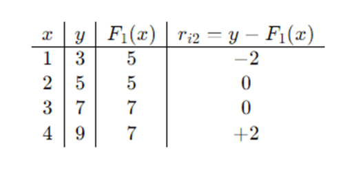
Step 0 — Initialize:

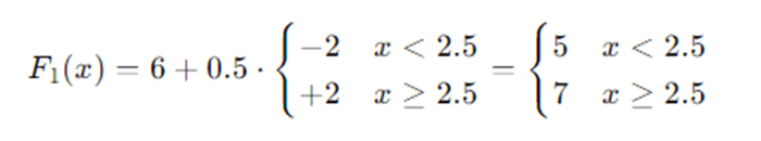
F₀(x)=mean(y)=(3+5+7+9)/4=6

Step 1 — Residuals (negative gradients):

r_i1=y_i−F₀(x_i)

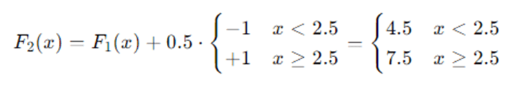
 Fit tree h₁​: With one split at x<2.5vs x≥2.5, leaf means are:

• Left leaf ℓL: residual mean =(−3+−1)/2=−2
• Right leaf ℓR: residual mean =(1+3)/2=+2

Line search (squared error simplifies to leaf means): γ1,ℓ are just these means.

Update with learning rate ν=0.5:

Step 2 — New residuals:

Fit h2​:

Another stump with the same split:

• Left leaf mean residual: (−2+0)/2=−1
• Right leaf mean residual: (0+2)/2=+1

Update:

We see predictions moving toward the true values. More rounds and slightly deeper trees would capture the linear pattern exactly. This illustrates the basic “fit residuals → add small correction” cycle.

Flow of Gradient Boosting

Advantages and Disadvantages of Gradient Boosting

Advantages

• High predictive accuracy on tabular data, often outperforming linear models and many neural nets with fewer samples.
• Flexible loss functions: squared, logistic, Huber, quantile, ranking—choose what matches your objective.
• Built-in feature interaction discovery: trees naturally capture nonlinearities and interactions without heavy feature engineering.
• Strong regularization toolkit: learning rate, early stopping, subsampling, tree constraints (depth, leaves, min samples), L1/L2 penalties (some libraries).
• Handles mixed data well: numeric, categorical (especially with CatBoost), missing values (depending on implementation).
• Interpretability aids: feature importance, SHAP values, partial dependence plots, interaction effects.

Disadvantages

• Training time can be longer than simpler models; sequential nature limits parallelization across boosting rounds (though per-tree parallelism exists).
• Parameter tuning matters: choosing learning rate, depth, estimators, and regularization is crucial; defaults aren’t always optimal.
• Overfitting risk if trees are deep, learning rate is high, or too many rounds without validation/early stopping.
• Less suited for extremely high-dimensional sparse problems (e.g., raw text) compared to linear models with strong regularization or specialized deep models.
• Concept drift sensitivity: when data distribution shifts, the model may need frequent retraining/monitoring.

Applications of Gradient Boosting

• Finance & Risk: credit scoring, fraud detection, default prediction, loss given default, risk ranking.
• Marketing & CRM: propensity modeling, churn prediction, uplift modeling, customer lifetime value, next-best-action.
• Operations & Forecasting: demand/price forecasting, capacity planning, predictive maintenance.
• Healthcare: readmission risk, diagnosis support, mortality prediction, length-of-stay estimation (with careful governance).
• Search & Ranking: learning-to-rank for search engines and recommenders (pairwise or listwise losses).
• Cybersecurity: anomaly detection in logs, malware scoring, intrusion detection.
• Insurance: claim severity/frequency, reserving, pricing.
• Manufacturing & IoT: sensor-based quality control, failure prediction.
• Energy: load forecasting, renewable output prediction.
• NLP tabular hybrids: features engineered from text (tf-idf, embeddings) combined with structured signals.

Practical Considerations and Tuning Tips

• Learning rate (ν) & estimators (M): smaller ν (e.g., 0.03–0.1) with larger M often generalizes better. Use early stopping on a validation set to pick M.
• Tree depth / leaves: depth 3–8 is common. Shallow trees encourage additive, smooth improvements; deeper trees capture complex interactions but risk overfit.
• Subsampling (stochastic GBM): use a row subsample (e.g., 0.6–0.9) to reduce variance and speed up training; many libraries also support column subsampling per tree/level/split.
• Regularization:
  • min_samples_leaf, min_child_weight, min_data_in_leaf  guard against tiny leaves.
  • L1/L2 penalties on leaf weights (implementation-dependent).
  • Monotonic constraints if you require business-logic consistency (e.g., price shouldn’t decrease predicted demand beyond limits).
• Handling categorical features:
  • One-hot encoding for low cardinality.
  • Target/statistical encoding (with leakage control) for high cardinality.
  • CatBoost handles categorical features natively with ordered statistics.
• Imbalanced classification:
  • Adjust scale_pos_weight or class weights; try focal/weighted losses.
  • Evaluate with AUC-PR, F1, cost-sensitive metrics, not accuracy alone.
• Diagnostics:
  • Use learning curves and validation curves.
  • Check feature importance (gain, split count, SHAP).
  • Monitor overfit (train vs. valid loss diverging).
  • Investigate calibration for probabilities (Platt, isotonic), especially in classification.

Conclusion

Gradient Boosting turns a simple idea—fix your mistakes a bit at a time—into an exceptionally capable modeling framework. By optimizing a loss through functional gradient descent, and expressing corrections with regularized, shallow trees, GBMs capture rich nonlinear patterns while staying reasonably interpretable and controllable. With thoughtful tuning (learning rate, depth, regularization, subsampling) and sound validation (early stopping), gradient boosting delivers state-of-the-art performance on many real-world, structured datasets. Whether you’re building a churn model, a risk score, or a ranking function, GBMs deserve a prominent place in your toolkit.

Frequently Asked Questions (FAQs)

How is Gradient Boosting different from XGBoost, LightGBM, and CatBoost?

Answer: Gradient Boosting is the general algorithmic idea. XGBoost, LightGBM, and CatBoost are high-performance implementations with engineering optimizations (histogram-based splits, sparsity awareness, parallelism), additional regularization, and specialized handling (e.g., categorical features in CatBoost). The core principle—additive training of trees on negative gradients—remains the same.

What hyperparameters matter most?

Answer: Typically learning rate, number of estimators, and tree complexity (depth/max leaves) dominate. Subsampling, ℓ1/ℓ2 ​ regularization on leaf weights, and minimum samples per leaf also matter. Start with a modest depth (e.g., 4–6), learning rate 0.05–0.1, and use early stopping to select estimators.

How do I avoid overfitting?

Answer: Use a validation set with early stopping, keep trees shallow, reduce the learning rate, subsample rows/columns, and increase min samples per leaf or min child weight. Monitor the validation loss/metric and stop when it stops improving.

Can Gradient Boosting output calibrated probabilities?

Answer: For logistic loss, outputs are in log-odds space and translate to probabilities via the logistic function. Calibration is usually decent but may benefit from post-hoc calibration (isotonic/Platt scaling), especially when class imbalance or distribution shift is present.

When should I prefer Random Forests or linear models instead?

Answer: Prefer Random Forests when you need simplicity, robustness with minimal tuning, or high parallelism; they shine on noisy data with weaker signal. Choose linear models when relationships are largely linear, features are extremely high-dimensional/sparse (e.g., text), or you need a very fast, interpretable baseline.