Girvan–Newman Algorithm

Table of Contents

What is the Girvan–Newman Algorithm?

The Girvan–Newman (GN) algorithm is a classic community detection method for networks (graphs). It identifies clusters (communities) by iteratively removing edges that act as “bridges” between groups. Instead of clustering nodes directly, GN focuses on edge betweenness centrality—a measure of how many shortest paths between node pairs flow through an edge. Edges with high betweenness are presumed to connect otherwise dense subgraphs; removing them gradually reveals community structure.

Introduction to Girvan–Newman

Community detection aims to partition a graph into subsets of nodes with dense internal connections and sparse external connections. Early methods emphasized node-centric measures or global partitions (like spectral cuts). Girvan–Newman (2002) reframed the problem through an edge-centric lens:

Key intuition: Edges that lie between communities carry a disproportionate share of shortest paths.
Strategy: Compute edge betweenness for all edges, remove the highest-betweenness edge(s), recompute betweenness on the modified graph, and repeat.
Stopping rule: Either stop when a desired number of communities appears, or track a quality score (often modularity, Q) and select the partition with the best score observed during the sequence of removals.

The algorithm is conceptually simple but computationally intensive. It’s still a foundational technique—useful as a teaching tool, for small to medium graphs, and as a baseline against which faster methods (e.g., Louvain, Leiden) are compared.

The Girvan–Newman Algorithm in Detail

3.1 Graph setup and notation

Graph G=(V,E) with ∣V∣=n nodes and ∣E∣=m edges.
Undirected, unweighted graphs are standard in the basic version, though weighted variants exist.
Let A be the adjacency matrix; k_i is the degree of node i.

3.2 Edge betweenness centrality

For an edge e∈E, edge betweenness CB(e) is:

Where:

σ_st is the number of shortest paths between nodes s and t,
σ_st(e) is the number of those shortest paths that pass through edge eee.

Interpretation: If many shortest paths must traverse e, that edge likely sits between communities and has high CB(e).

Computation: In unweighted graphs, σ_st and path dependencies can be computed efficiently with BFS from each source node (Brandes’ algorithm idea). For weighted graphs, Dijkstra’s algorithm replaces BFS.

3.3 Modularity Q (optional scoring/selection)

Modularity measures the quality of a partition into communities {C₁,C₂,…,C_K}:

A_ij is adjacency (1 if edge, else 0, unweighted case),
k_i,k_j are degrees,
m=∣E∣,
c_i is the community label of node i,
δ(⋅,⋅) is 1 when nodes i and j fall in the same community and 0 otherwise.

Interpretation: Q compares the fraction of edges inside communities against what we expect in a random graph with the same degree sequence. Higher Q indicates stronger community structure.

3.4 Algorithm outline

Compute edge betweenness CB(e) for every edge e∈E.
Identify and remove the edge(s) with maximum CB(e).
Recompute CB(e) on the (now modified) graph because removal may shift shortest paths.
Record partitions as the graph splits into connected components. Optionally compute modularity Q for each partition.
Repeat steps 1–4 until no edges remain (or until a target number of communities is reached).
Select the best partition, often the one that maximizes modularity Q, or the one matching a user-chosen community count.

3.5 Complexity

A single full computation of edge betweenness using BFS from all nodes takes O(nm) time for unweighted graphs.
Because GN recomputes betweenness after every removal, the worst-case complexity is roughly O(m²ⁿ) for unweighted graphs (and worse for weighted when using Dijkstra).
Therefore, GN is best suited for small to medium graphs (hundreds to low thousands of nodes/edges).

Step-by-Step Explanation

Step 1: Compute edge betweenness.

Start with the full graph. For every pair of nodes, find shortest paths; count how many pass through each edge. Aggregate over all pairs to obtain CB(e) for each edge. In practice, we don’t enumerate pairs explicitly; we run a BFS from each node s (or Dijkstra for weighted graphs) and compute dependency values that roll up the contributions to σst(e). Intuitively, edges that connect dense regions tend to carry many shortest paths, leading to high CB(e).

Step 2: Remove the most “between” edge(s).

Identify the edge(s) with maximal CB(e). Removing them is akin to cutting the tightest “bridge” between communities. If there are ties, we can remove all co-maximal edges simultaneously or break ties arbitrarily—either way, the algorithm proceeds by progressively weakening inter-community connections.

Step 3: Recompute betweenness on the updated graph.

Edge betweenness centrality is context-dependent: once a bridging edge is removed, the set of shortest paths changes. New edges may become the next bridges. Recomputing ensures the algorithm remains responsive to the graph’s evolving topology.

Step 4: Track connected components and (optionally) modularity.

As edges disappear, the graph may split into multiple connected components—these are the communities at that iteration. If we are optimizing by modularity Q, compute Q for each partition encountered. Often, Q rises to a peak and then falls as we over-fragment the graph. The partition at the peak Q is a common choice.

Step 5: Iterate until a stopping criterion is met.

Continue removing edges and re-evaluating until we’ve reached the target number of communities, the maximum modularity, or until the graph is fully disconnected. The algorithm produces a dendrogram-like sequence of splits (a hierarchy of partitions). Users can pick a level appropriate to their domain.

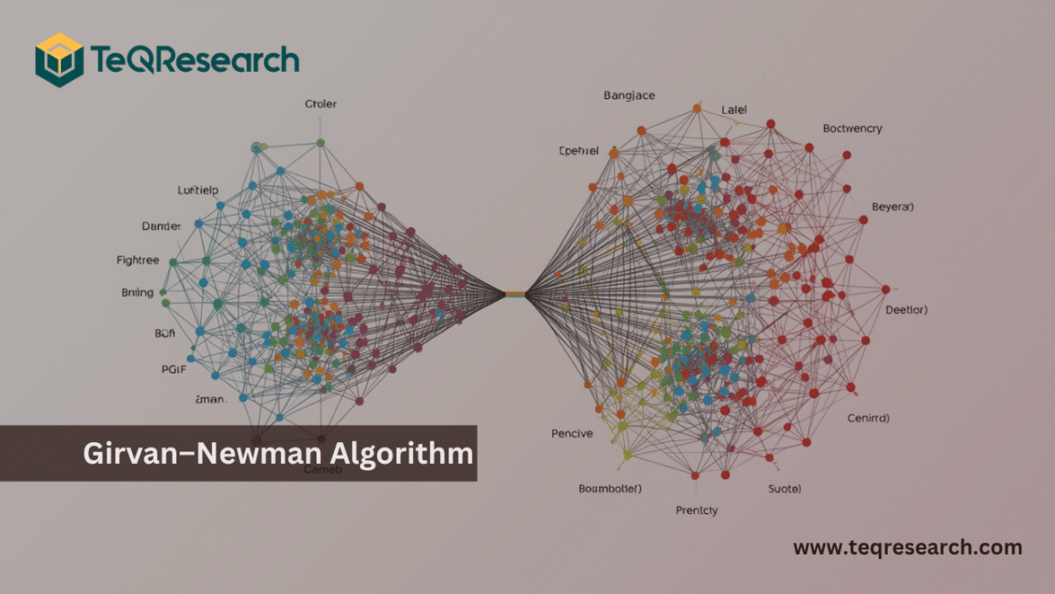
Example: How Girvan–Newman Works

Consider a simple graph with two dense clusters connected by one bridge. Within each cluster, many triangles and short cycles create multiple alternative shortest paths; between clusters, almost every shortest path must cross the bridge. Consequently, the bridge edge has the highest edge betweenness.

Initial state: Compute CB(e) for all edges. The bridge edge scores highest, because all cross-cluster shortest paths funnel through it.
First removal: Remove the bridge edge. The graph splits into two connected components—each roughly corresponds to a cluster/community.
Subsequent steps: If we kept removing edges, each community would further fragment; modularity typically peaks right after the bridging edges are removed and before we start tearing apart the internal structure of the communities.

To visualize this, I created a simple diagram that highlights the bridging edge as the likely highest-betweenness edge and annotates the GN steps.

Advantages and Disadvantages

Advantages

Conceptually intuitive: Focuses on the idea that bridges connect communities; removing them reveals clusters.
Interpretable steps: Each removal has a rationale (“this edge carries many shortest paths”).
Produces a hierarchy: The sequence of removals yields multiple partitions; you can select the resolution you prefer.
Quality-aware via modularity: GN can be paired with modularity to pick the “best” partition among many.
Good baseline: Despite being slower than modern methods, GN remains a gold-standard baseline for small graphs and teaching.

Disadvantages

Computationally expensive: Recomputing edge betweenness after every removal leads to O(m²ⁿ) time complexity, limiting scalability.
Sensitivity to shortest paths: Betweenness centrality depends on shortest paths; in graphs with many near-shortest alternatives or weighted edges with noise, rankings may be unstable.
Resolution limits (via modularity): If modularity is used to select the partition, it suffers from the resolution limit—small communities may be missed.
Edge removals can be brittle: In very sparse or tree-like graphs, removing a single edge can isolate nodes prematurely; careful interpretation is needed.
Not ideal for dynamic graphs: GN recomputations from scratch are expensive when the network changes frequently.

Applications of Girvan–Newman

Social network analysis: Discovering friend groups, organizational subunits, or influencer-bridged clusters in collaboration networks.
Biological networks: Finding functional modules in protein–protein interaction or gene co-expression networks.
Information networks: Detecting topical clusters in citation or hyperlink graphs.
Infrastructure and transport: Identifying critical inter-community links (bridges) in road, power, or airline networks—useful for resilience analysis.
Marketing & recommendation: Segmenting customers or products into communities to tailor campaigns or cross-sell strategies.
Security/forensics: Flagging bridge edges or nodes that connect otherwise separate groups, potentially indicating brokers or anomalous connectors.
Education & research: As a teaching tool for network science, demonstrating the relationship between shortest paths, bottlenecks, and community structure.

Conclusion

The Girvan–Newman algorithm is a seminal, edge-centric approach to community detection. By iteratively removing high-betweenness edges and optionally evaluating modularity, GN exposes underlying clusters in a network and provides a hierarchical view of splits. While its computational cost limits its use on large graphs, its transparency and interpretability make it invaluable for small to medium networks, exploratory analysis, and pedagogy. In practice, GN can complement faster algorithms: use GN to verify, explain, or illustrate community structure, then deploy scalable methods (e.g., Louvain/Leiden) for big data.

Frequently Asked Questions (FAQs)

How is edge betweenness different from node betweenness?

Edge betweenness counts the fraction of shortest paths that pass through an edge, whereas node betweenness does the same for nodes. GN uses edge betweenness because it directly targets links that connect communities; removing a high-betweenness edge is a natural way to split communities apart.

Do I need to remove one edge at a time, or can I remove all ties?

Both are used in practice. If several edges share the maximum betweenness, removing them together can speed things up and mirrors the idea that multiple bridges may be equally critical. Just remember to recompute betweenness after each removal round.

How do I choose the “right” number of communities?

A common approach is to compute modularity Q for each partition encountered during the GN process and select the partition with maximum Q. Alternatively, you can pick a community count that aligns with domain knowledge or stability diagnostics (e.g., where partitions change minimally across iterations).

Can Girvan–Newman handle weighted graphs?

Yes—replace BFS with Dijkstra’s algorithm to compute shortest paths with edge weights. You then compute edge betweenness using weighted shortest paths. Be aware that weights change the notion of “shortest,” and results may be more sensitive to noise.

Is Girvan–Newman suitable for large networks?

Not typically. The repeated recomputation of betweenness makes GN slow for large graphs. For big networks, prefer faster heuristics (e.g., Louvain or Leiden) and use GN on smaller subgraphs for interpretability or validation.