What is Cellular Evolutionary Algorithm?
A Cellular Evolutionary Algorithm (CEA) is a type of evolutionary algorithm in which individuals in the population are arranged in a structured spatial topology—typically a two-dimensional grid—and interact primarily with their local neighbors rather than with the entire population. This localized interaction model distinguishes CEAs from classical Genetic Algorithms (GAs), where selection and reproduction are generally performed globally. In a CEA, each individual occupies a “cell” in a lattice (grid), and evolutionary operations such as selection, crossover, and mutation occur within a small neighborhood (e.g., von Neumann or Moore neighborhood). This spatial distribution promotes slow diffusion of genetic material across the population, thereby maintaining diversity and preventing premature convergence. In essence, a Cellular Evolutionary Algorithm introduces spatial structure into evolutionary computation, enabling controlled information propagation and enhanced exploration-exploitation balance.
Introduction of Cellular Evolutionary Algorithm
Cellular Evolutionary Algorithms belong to the broader family of Evolutionary Computation (EC) techniques, which are inspired by natural evolution. These include:
- Genetic Algorithms (GAs)
- Evolution Strategies (ES)
- Genetic Programming (GP)
- Differential Evolution (DE)
Traditional evolutionary algorithms treat the population as panmictic (fully mixed), meaning any individual can interact with any other. While this accelerates convergence, it often leads to:
- Loss of diversity
- Premature convergence
- Local optima trapping
To overcome these limitations, researchers introduced structured population models, among which CEAs are particularly significant.
The concept of structured populations was influenced by:
- Cellular automata models
- Distributed evolutionary algorithms
- Parallel computing frameworks
CEAs became especially popular in parallel computing environments because each cell can evolve independently while interacting locally, making them naturally suited for distributed systems and GPUs.
Detailed Cellular Evolutionary Algorithm
3.1 Basic Representation
Let:
- P(t)= {x1(t),x2(t),…,Xn(t)} be the population at generation t
- Each individual xi(t)ÎRd (for continuous optimization)
- The population is arranged in a 2D grid of size m×n, where N=m×n
Each individual occupies a cell (i,j).
3.2 Neighborhood Structure
Define a neighborhood function:

Common neighborhood types:
- Von Neumann Neighborhood

- Moore Neighborhood

3.3 Fitness Evaluation
Each individual is evaluated using an objective function:

For minimization:

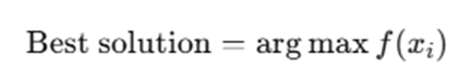
For maximization:
3.4 Selection
Selection occurs within the neighborhood:

Example: Tournament selection within neighborhood:

where S⊆Ni,j
3.5 Crossover
Given two parents xa and xb:
Single-point crossover:

For real-valued vectors:

where α∈[0,1]
3.6 Mutation
For real-valued mutation:
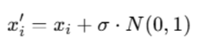
Where:
- σ = mutation strength
- N(0,1) = Gaussian random variable
3.7 Replacement
Replacement is typically local:

This ensures steady diffusion of better solutions.
3.8 Algorithm Steps
- Initialize population in grid.
- Evaluate fitness.
- For each cell:
- Select parents from neighborhood.
- Apply crossover.
- Apply mutation.
- Evaluate offspring.
- Replace if better.
- Repeat until termination criterion is met.
A Cellular Evolutionary Algorithm begins by initializing a structured population arranged on a two-dimensional lattice. Each cell in the grid contains one candidate solution to the optimization problem. Unlike traditional evolutionary algorithms, interaction is restricted to a defined local neighborhood. This spatial restriction plays a fundamental role in maintaining diversity and controlling convergence speed. After initialization, each individual is evaluated using a predefined fitness function. The fitness function quantifies how good a candidate solution is relative to the optimization objective. Once fitness values are computed, evolutionary operations begin.
For every individual in the grid, a subset of neighboring individuals is identified. This subset may follow a von Neumann or Moore configuration. Selection occurs only within this neighborhood, ensuring localized competition. Tournament selection or roulette wheel selection may be used to choose parents. Following selection, crossover is applied to generate new offspring. In binary problems, this may involve exchanging segments of bit strings. In continuous problems, arithmetic recombination is commonly applied. The offspring inherits genetic material from both parents.
Mutation introduces random perturbations to prevent stagnation and improve exploration. For real-valued representations, Gaussian mutation is often used. This step ensures the algorithm does not converge prematurely. The newly generated offspring is evaluated. If it outperforms the current individual occupying the cell, replacement occurs. Otherwise, the original individual remains. Because replacement is local, improvements propagate gradually through the grid rather than instantly dominating the population.
This process repeats for multiple generations until a stopping criterion—such as maximum iterations or acceptable fitness—is met.
Example of How Cellular Evolutionary Algorithm Works
Example Problem: Minimize Function
f(x)=x2
Assume a 3×3 grid:
Initial population:
| 4 | -3 | 5 |
| 2 | -1 | 3 |
| 6 | -4 | 1 |
Each cell evaluates f(x).
Suppose cell (2,2) = -1:
- Neighborhood: {2, -1, 3, -3}
- Best neighbor: -1
- Crossover and mutation generate 0.2
- Since f(0.2)=0.04<f(−1)=1, replacement occurs.
Gradually, 0 spreads across the grid.

Advantages and Disadvantages
Cellular Evolutionary Algorithms (CEAs) incorporate a spatially structured population, typically arranged in a grid, where individuals interact primarily with their local neighbors. This design significantly influences their convergence behavior, diversity preservation, and computational characteristics compared to traditional panmictic Genetic Algorithms (GAs). Below is a structured explanation of the key advantages and disadvantages of CEAs.
Advantages
- Maintains Population Diversity: One of the primary strengths of CEAs is their ability to preserve genetic diversity within the population. Because individuals interact only with nearby neighbors rather than the entire population, superior solutions spread gradually across the grid instead of immediately dominating it. This slow diffusion of information prevents rapid homogenization and allows multiple promising regions of the search space to evolve simultaneously. Maintaining diversity is especially critical in solving complex, multimodal optimization problems.
- Prevents Premature Convergence: Premature convergence occurs when an algorithm settles on a local optimum before adequately exploring the search space. In traditional GAs, global selection mechanisms can quickly amplify moderately good solutions, leading to diversity loss and stagnation. CEAs reduce this risk by restricting competition to local neighborhoods. This localized selection allows different regions of the grid to evolve semi-independently, significantly decreasing the likelihood of the entire population converging prematurely to a suboptimal solution.
- Better Exploration of Search Space: The grid-based structure enables distributed search behavior. Different sections of the population can explore different regions of the solution landscape at the same time. While some neighborhoods exploit high-quality solutions, others continue exploring alternative areas. This balance between exploration and exploitation enhances robustness and improves the algorithm’s ability to handle nonlinear, high-dimensional, and multimodal objective functions.
- Naturally Parallelizable: CEAs are inherently suitable for parallel and distributed computing environments. Since each cell interacts mainly with its local neighbors, most evolutionary operations can be executed independently. This makes CEAs highly compatible with multi-core processors, GPU systems, distributed clusters, and high-performance computing architectures. As a result, they scale efficiently for large-scale optimization problems.
- Controlled Convergence Speed : Unlike traditional evolutionary algorithms that may converge too quickly, CEAs offer a more controlled and gradual convergence process. The local propagation of superior solutions ensures steady improvement over generations without sudden dominance by a single individual. This controlled convergence often results in higher-quality solutions, particularly in rugged or deceptive fitness landscapes.
Disadvantages
- Slower Convergence Compared to Panmictic GA: Because information spreads locally rather than globally, CEAs often converge more slowly than traditional Genetic Algorithms. While this slower convergence improves diversity and exploration, it may increase the number of generations required to reach optimal solutions, particularly for simple or unimodal problems where rapid convergence would be beneficial.
- Requires Careful Neighborhood Design : The performance of a CEA strongly depends on the chosen neighborhood structure (such as von Neumann or Moore neighborhoods). A small neighborhood maintains diversity longer but slows convergence, while a larger neighborhood accelerates convergence but reduces diversity. Improper neighborhood configuration can negatively impact performance, making careful design and experimentation necessary.
- Higher Computational Overhead: Maintaining a structured grid and performing neighborhood-based selection introduce additional computational complexity compared to managing a simple unstructured population. Operations such as neighbor identification, localized selection, and structured replacement increase implementation complexity and memory usage.
- Parameter Tuning Complexity: CEAs involve several parameters that must be carefully adjusted, including grid size, neighborhood shape, crossover probability, mutation rate, and selection pressure. The optimal configuration often depends on the specific problem being solved. Improper tuning can degrade performance, making parameter selection a challenging task.
- Grid Structure May Limit Interaction: While spatial restriction helps preserve diversity, it can also delay beneficial genetic combinations. If high-quality solutions are located far apart in the grid, it may take many generations before they interact through gradual diffusion. This limitation may slow convergence or reduce efficiency in certain optimization problems.
Applications of Cellular Evolutionary Algorithm
Cellular Evolutionary Algorithms (CEAs) are widely used across scientific, engineering, and industrial domains because of their ability to maintain diversity, prevent premature convergence, and efficiently explore complex search spaces. Their grid-based population structure enables distributed search and gradual information diffusion, making them especially suitable for nonlinear, high-dimensional, and multimodal optimization problems.
- Engineering Optimization: In engineering, CEAs are applied to structural design optimization, mechanical parameter tuning, aerodynamic shape optimization, and power system optimization. They help minimize weight, cost, or energy consumption while satisfying safety and performance constraints. Their ability to explore multiple design alternatives simultaneously makes them effective for complex systems with nonlinear constraints.
- Image Processing: CEAs are used in feature selection, image segmentation, edge detection, and object recognition parameter tuning. By maintaining diverse candidate solutions, they effectively handle high-dimensional image data and improve accuracy in segmentation and classification tasks.
- Machine Learning: In machine learning, CEAs optimize neural network weights, tune hyperparameters, and perform feature subset selection. Since they do not require gradient information, they are suitable for non-convex optimization problems and help avoid premature convergence during model training and architecture search.
- Robotics: CEAs support path planning, swarm coordination, motion optimization, and control parameter tuning in robotic systems. Their localized interaction model resembles swarm intelligence, making them effective for distributed and autonomous robotic applications.
- Bioinformatics: In bioinformatics, CEAs are applied to gene expression analysis, protein structure prediction, sequence alignment, and drug discovery optimization. Their diversity-preserving mechanism helps navigate complex multimodal biological fitness landscapes.
- Scheduling Problems: CEAs are widely used in job shop scheduling, resource allocation, task scheduling, and timetable optimization. Their robustness helps manage combinatorial complexity and improve solution quality in constraint-based scheduling problems.
- Combinatorial Optimization: CEAs are applied to classic problems such as the Traveling Salesman Problem (TSP), Knapsack Problem, vehicle routing, and graph coloring. By maintaining diversity longer than traditional evolutionary algorithms, they perform particularly well in multimodal combinatorial problems where multiple local optima exist.
Conclusion
The Cellular Evolutionary Algorithm (CEA) represents a significant advancement over classical evolutionary algorithms by incorporating a spatially structured population model. Unlike traditional Genetic Algorithms (GAs), where individuals interact globally, CEAs organize individuals in a grid and restrict interactions to local neighborhoods. This spatial constraint fundamentally changes the evolutionary dynamics by enabling gradual information diffusion rather than rapid global dominance. Through localized interaction, CEAs effectively balance exploration (searching new regions of the solution space) and exploitation (refining promising solutions). The controlled propagation of superior individuals reduces the risk of premature convergence while preserving genetic diversity across generations. This makes CEAs particularly well-suited for complex, nonlinear, high-dimensional, and multimodal optimization problems where maintaining diverse candidate solutions is critical.
Although CEAs may converge more slowly than traditional panmictic GAs due to their localized selection mechanism, they often produce higher-quality and more robust solutions. Their structured design also aligns naturally with parallel and distributed computing architectures such as multi-core processors and GPUs, making them highly scalable for large-scale computational tasks. As optimization challenges continue to expand in fields such as artificial intelligence, engineering design, robotics, bioinformatics, and data science, Cellular Evolutionary Algorithms remain a powerful, flexible, and scalable methodology capable of addressing increasingly complex problem landscapes.
Frequently Asked Questions (FAQs)
1. What makes Cellular Evolutionary Algorithm different from Genetic Algorithm?
The primary difference lies in population structure and interaction. In a traditional Genetic Algorithm, individuals can interact with any other member of the population (global interaction). In contrast, a Cellular Evolutionary Algorithm restricts interaction to local neighborhoods within a structured grid, leading to slower but more controlled information diffusion.
2. Why is spatial structure important in CEA?
Spatial structure preserves diversity by preventing a single high-fitness individual from immediately dominating the entire population. This gradual diffusion of genetic material reduces premature convergence and enhances the algorithm’s ability to explore complex search spaces.
3. What types of problems are best suited for CEA?
CEAs are particularly effective for multimodal optimization problems, combinatorial optimization tasks, large-scale engineering design problems, and high-dimensional nonlinear systems where maintaining diversity and avoiding local optima are essential.
4. Can CEA be parallelized?
Yes. CEAs are naturally parallelizable because each cell primarily interacts with its local neighbors. This independence makes them well-suited for parallel computing environments, including GPUs, distributed systems, and high-performance computing clusters.
5. What neighborhood structure is best?
The optimal neighborhood structure depends on the problem. Moore neighborhoods allow broader interaction and faster convergence, while von Neumann neighborhoods promote slower diffusion and stronger diversity preservation. The choice should be guided by the desired balance between exploration and exploitation.