Latent Semantic Analysis (LSA) is a foundational technique in natural language processing and information retrieval that uncovers hidden (latent) relationships between words and documents. It transforms raw text into a lower-dimensional semantic space where synonymous or related words and documents cluster together — even when they don’t share exact word overlap. LSA powers tasks like document similarity, query expansion, topic extraction, and semantic search. This post explains LSA from first principles, walks through the algorithm step-by-step with formulas, gives a worked example and a diagram, and discusses advantages, disadvantages, and real-world applications. By the end you’ll have a clear, mathematically grounded understanding of how LSA works and when to use it.

What is Latent Semantic Analysis?

Latent Semantic Analysis (LSA), also called Latent Semantic Indexing (LSI) when applied to retrieval systems, is a method that maps text (terms and documents) into a continuous vector space that captures the principal patterns of association between terms and documents. The core idea: observed word usage patterns across documents are noisy indicators of deeper semantic concepts. LSA uses linear algebra — specifically the singular value decomposition (SVD) — to discover those latent concepts and to produce a compact representation of documents and terms that emphasizes conceptual similarity over mere surface-level lexical overlap.

Key intuitions:

• Words that appear in similar contexts are likely to be semantically related.
• Documents that use similar groups of words are likely to be about similar topics.
• Reducing dimensionality filters noise and reveals the dominant semantic structure.

Introduction to Latent Semantic Analysis

Historically, LSA originated in the early 1990s (Deerwester et al., 1990) as a response to limitations in keyword-based retrieval: queries and documents often use different words to express the same idea (synonymy), while the same word can have multiple meanings (polysemy). LSA addresses synonymy by projecting words and documents into a lower-dimensional space where semantically related items are close even if they share few surface words. It mitigates polysemy because multiple senses of a word are blended into principal components that reflect dominant usage patterns.

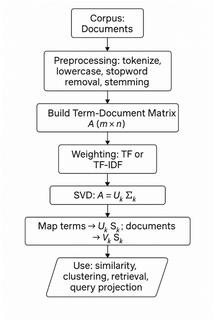
The standard pipeline for LSA:

1. Build a term-document matrix A.
2. Optionally apply weighting (e.g., TF-IDF) to entries.
3. Compute the singular value decomposition A=UΣV⊤.
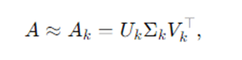
4. Keep only the top k singular values and corresponding vectors to form a rank-k approximation A_k=U_kΣ_kV_k^⊤ ​.
5. Use the low-dimensional coordinates of terms and documents for similarity, clustering, or retrieval.

LSA is unsupervised, domain-agnostic, and relatively simple to implement using standard linear algebra libraries. However, it relies on linear assumptions and ignores word order and word morphology.

Detailed Latent Semantic Analysis — Algorithm

Below I give the formal mathematical statement of LSA, with the key formulas used at each step.

3.1: Term–Document Matrix Construction

Given a corpus with m unique terms (words) and n documents, build matrix A∈R_m×n where each cell a_ij ​ measures the association between term iii and document j.

Common choices for a_ij ​:

• Raw term frequency: a_ij=tf_ij (count of term i in document j).
• Term frequency–inverse document frequency (TF–IDF):

Where df_i is the number of documents containing term i.

• Log-scaled: a_ij=1+log⁡(tf_ij) when tf_ij>0, else 0.

TF–IDF example formula:

(Adding 1 to avoid division by zero and to smooth small corpora.)

3.2: Singular Value Decomposition (SVD)

Perform SVD on A:

A=UΣV^⊤.

Components:

• U∈R_m×m— columns are orthonormal left singular vectors (term eigenvectors).
• Σ∈R_m×n— diagonal matrix with singular values σ1≥σ2≥⋯≥0.
• V∈R_n×n— columns are orthonormal right singular vectors (document eigenvectors).

In practice, since A is typically tall or wide, we compute a reduced SVD. If we want the top k components:

Where,

• U_k∈R^m×k (first k columns of U),
• Σ_k∈R^k×k (top k singular values on diagonal),
• V_k∈R^n×k (first k columns of V).

This is the best rank-k approximation of A in the least-squares (Frobenius norm) sense by the Eckart–Young theorem.

3.3: Dimensionality Reduction and Representations

• Term vectors in latent space: rows of U_kΣk ​. For term i, its k-dimensional latent vector is the i_th row of U_kΣk ​, often denoted t_i∈R_k.
• Document vectors in latent space: rows of V_kΣ_k ​. For document j, its vector is the j_th row of V_kΣk, denoted d_j∈R_k.

Equivalently, columns of U_k ​ and V_k ​ serve as basis directions; scaling by Σ_k provides coordinate magnitudes.

3.4: Similarity Computation

For semantic similarity between documents d_p​ and d_q, compute the cosine similarity in the reduced space:

Similarly, for a query represented as a term vector q mapped into latent space, compute similarity against document vectors.

3.5: Query Projection

Given a query q expressed in the original term space (size m), project into the latent space using:

More concretely, using the relation A≈U_kΣ_kV_k⊤​, the canonical projection is:

Then compute cosine similarity between q_k​ and document coordinates d_j = σ_iv_K^⊤, or equivalently transform both to the same coordinate frame before comparison.

3.6: Reconstruction & Interpretation

The rank-k reconstructed matrix A_k  approximates original co-occurrence:

Each term σ_iu_iv_i^⊤ captures a latent concept; larger σ_i correspond to stronger concepts present in the corpus.

Step-by-step LSA

First, LSA begins by transforming raw text into a numeric form: the term–document matrix. Each row corresponds to a distinct term (often after lowercasing, stop-word removal, and optional stemming), and each column corresponds to a document. The matrix entries capture the importance of a term in a document; basic options include raw term counts (TF) or TF–IDF weights which dampen ubiquitous words and emphasize discriminative words. Proper weighting is important because raw counts can over-emphasize long documents and very frequent words; TF–IDF often yields better semantic structure for LSA.

Once the matrix A is constructed, the algorithm performs singular value decomposition (SVD). SVD factorizes A into three matrices U, Σ, and V⊤. Intuitively, SVD rotates and scales the original coordinate system so that the axes are ordered by how much variance (information) they explain in the data. The left singular vectors in U capture principal term patterns, the right singular vectors in V capture principal document patterns, and the singular values on the diagonal of Σ measure the importance of each pattern.

The next crucial step is truncation: choose a target dimension k (usually far smaller than the original rank) and keep only the top k singular values and corresponding singular vectors. This produces a compact approximation A_k=U_kΣ_kV_k⊤ ​. This dimensionality reduction both compresses the data and denoises it: components associated with small singular values typically correspond to idiosyncratic noise or rare word usages and are removed. Choosing k is a trade-off: too small and you lose important semantic distinctions; too large and you retain noise and overfit.

Terms and documents are then represented in the k-dimensional semantic space. Terms map to row vectors from UkΣk ​, and documents map to row vectors from VkΣk. Importantly, queries — represented as term-frequency vectors — are projected into the same latent space, commonly using qk=Σk−1Uk⊤q (then optionally scaled). Similarity computations (e.g., cosine similarity) in this reduced space reveal latent relationships: documents that did not share exact words may be close because they express similar underlying concepts.

Finally, LSA outputs can be used in several tasks: ranking documents for query retrieval, clustering documents or terms, performing dimensionality reduction before supervised learning, or identifying dominant topics. Interpretability can be achieved by inspecting top-weighted terms in each singular vector (principal component), although each component is a linear blend and may not correspond to a single interpretable topic.

Example: How Latent Semantic Analysis Works

Let’s illustrate LSA with a compact, conceptual example (keeps numerical complexity low while demonstrating process). Suppose we have 4 short documents:

• Doc1: “cats like milk”
• Doc2: “cats like tuna”
• Doc3: “dogs like bone”
• Doc4: “dogs chase cats”

Vocabulary: {cats, dogs, like, milk, tuna, bone, chase} — 7 terms. Build the term–document matrix A of size 7×4 with raw term frequency:

Index rows in this order: 1:cats, 2:dogs, 3:like, 4:milk, 5:tuna, 6:bone, 7:chase.

Then:

Columns correspond to Doc1..Doc4.

We could (and usually should) apply TF–IDF weighting; for this toy example we proceed conceptually. Apply SVD to A:

A=UΣV^⊤.

Computing SVD numerically is routine with libraries; conceptually the SVD will find patterns such as “cat-related” vs “dog-related” and “like” as a shared behavior term. If we choose k=2, the rank-2 approximation A2​ captures the principal two latent concepts, perhaps roughly: (1) pet-food preference (cats/dogs like X) and (2) inter-species action (dogs chase cats).

In the reduced space:

• Doc1 and Doc2 (cats + food) will be near each other.
• Doc3 (dogs + bone) will be closer to Doc1/Doc2 along the “like” dimension but separated along the animal dimension.
• Doc4 (dogs chase cats) will be close to dogs but also to cats because of the “chase” relation — capturing an unexpected connection.

This small example shows how LSA can identify the shared concept “like” linking cat and dog documents and reveal nuanced relationships even when documents do not share all words.

Concrete small-matrix example — conceptual numeric steps (no heavy arithmetic)

Because SVD involves square roots and orthonormal bases, exact hand computation is lengthy. Practically, you compute SVD using numerical libraries (NumPy, SciPy). The crucial operations to understand are: compute Uk,Σk,Vk ​, then obtain document vectors d_j = σ_iv_K^⊤,  and compute cosine similarities.

Below is a short practical outline you can use as a starting point.

1. Preprocessing: tokenize, lowercase, remove stopwords, optional stemming/lemmatization.
2. Build term-document matrix A, apply TF–IDF.
3. Use a library SVD (truncated):

from sklearn.feature_extraction.text import TfidfVectorizer

from sklearn.decomposition import TruncatedSVD

# docs: list of document strings

vec = TfidfVectorizer(max_features=20000, stop_words=’english’)

A = vec.fit_transform(docs)  # sparse m x n (terms x docs) or n x m depending on implementation

k = 200

svd = TruncatedSVD(n_components=k)

A_k = svd.fit_transform(A)  # returns n_docs x k document vectors

# For term vectors, inspect svd.components_.T scaled by singular values

4. Compute cosine similarity in reduced space for retrieval.

Advantages and Disadvantages of Latent Semantic Analysis

Advantages

• Reduces synonymy problems: Documents that use different words for the same concept become close in latent space.
• Noise reduction: Dimension truncation filters out idiosyncratic or noisy word usage.
• Unsupervised and domain-agnostic: No labeled data required; works for many text corpora.
• Mathematical optimality: SVD gives the best low-rank approximation in least-squares sense (Eckart–Young theorem).
• Compact representations: Low-dimensional vectors are efficient for storage, indexing, and downstream models.
• Simple pipeline: Conceptually straightforward and easy to implement with standard linear algebra packages.

Disadvantages

• Linear model: LSA captures linear correlations; it cannot model non-linear structure that more advanced methods (e.g., neural embeddings) capture.
• Interpretability limits: Singular vectors are linear combinations of terms and may be hard to interpret as clean topics.
• Choice of k: Selecting the number of dimensions k is empirical; poor choices hurt performance.
• Scalability: SVD on large term–document matrices can be computationally expensive (though truncated/randomized SVD and incremental methods mitigate this).
• Ignores word order and syntax: LSA is bag-of-words based — it discards word order and grammatical structure.
• Polysemy blending: Different senses of a word may be mixed into shared components, potentially reducing specificity.
• Sensitivity to preprocessing and weighting: Results depend strongly on how you preprocess text and weight the matrix (stopwords, stemming, TF–IDF choice).

Applications of Latent Semantic Analysis

LSA has been successfully applied across many NLP and information retrieval tasks:

• Information retrieval / Search engines: LSA (LSI) helps match queries with documents even when exact keywords differ.
• Document clustering & topic discovery: Low-dimensional vectors make clustering more robust and reveal latent topics.
• Recommender systems: Use document/term vectors to recommend related articles, papers, or products.
• Text summarization: Identify main semantic components and select representative sentences.
• Plagiarism detection: Detect semantically similar passages that use different wording.
• Semantic similarity and paraphrase detection: Compare sentences or short texts in latent space.
• Feature engineering: Use LSA vectors as features for supervised models (classification, regression).
• Cognitive modeling: LSA has been used as an explanatory model of human semantic memory and similarity judgments in psychology.
• Query expansion: Expand user queries with semantically related terms discovered in latent space.

While newer techniques like word2vec, GloVe, and transformer-based embeddings (BERT, GPT) have become popular due to their richer representations and ability to model context, LSA remains a lightweight, interpretable baseline and performs well in many constrained settings.

Conclusion

Latent Semantic Analysis is a powerful, mathematically principled technique for discovering latent structure in text corpora. By constructing a term–document matrix and applying singular value decomposition followed by dimensionality truncation, LSA reveals semantic patterns that help overcome simple keyword mismatches, reduce noise, and produce compact semantic representations for documents and terms. Its simplicity, unsupervised nature, and grounding in linear algebra make it an excellent tool for tasks ranging from search to topic discovery. However, LSA’s linearity, disregard for word order, and sensitivity to parameter choices mean it may not match performance of modern contextual embeddings in every use case. Still, LSA remains a valuable method — especially where interpretability, computational simplicity, or small-data robustness matter.

Frequently Asked Questions (FAQs)

How do I choose the number of dimensions k for LSA?

Choosing k is empirical. Common approaches: try multiple values (e.g., 50, 100, 200) and evaluate performance on a target task (retrieval accuracy, clustering coherence). Use explained variance / singular value decay as guidance: plot singular values and look for an “elbow” where marginal gains diminish. For small corpora, smaller k (20–100) often suffices; for large corpora, 200–500 may be appropriate. Cross-validation on downstream tasks is the safest method.

Should I use raw counts or TF–IDF before applying LSA?

TF–IDF is usually recommended because it downweights common words and highlights discriminative terms, improving the latent structure. Raw counts can bias SVD toward frequent terms and long documents. Try both and validate on your task.

Is LSA the same as topic modeling like LDA?

Not exactly. LSA is a linear algebra technique producing continuous latent dimensions (orthogonal bases). Latent Dirichlet Allocation (LDA) is a probabilistic generative model producing interpretable discrete topics as probability distributions over words. LDA often yields more interpretable topics, while LSA is mathematically simpler and sometimes better at capturing global structure.

How does LSA compare to word embeddings (Word2Vec, GloVe) and contextual models (BERT)?
Word2Vec/GloVe produce word-level embeddings trained to capture local co-occurrence patterns; they are non-linear in training but often still feed into linear operations. BERT and similar transformers produce contextualized embeddings sensitive to word order and context. These modern models typically outperform LSA on many semantic tasks but are heavier computationally. LSA remains a strong baseline for small/medium corpora or when interpretability and simplicity are priorities.

How can I scale LSA to very large corpora?

Use truncated or randomized SVD algorithms (e.g., Facebook’s randomized SVD, or algorithms in SciPy/Scikit-learn) that compute only top k singular vectors efficiently. Use sparse matrix representations to save memory. Incremental SVD or streaming SVD methods can handle data that doesn’t fit into memory. Dimensionality reduction (e.g., hashing, vocabulary trimming) can reduce problem size before SVD.