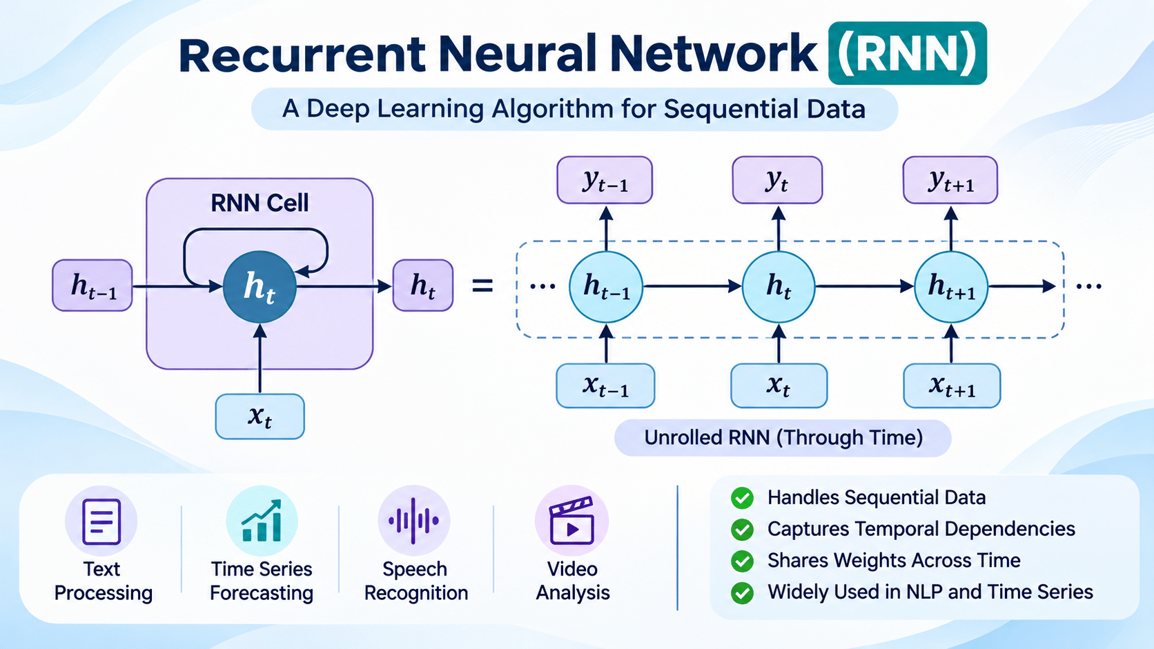
A Recurrent Neural Network (RNN) is a neural network architecture designed to process sequential information by carrying a hidden state from one time step to the next. This feedback mechanism allows the network to use information from earlier elements of a sequence when interpreting the current element. RNNs have been applied to language modelling, time-series forecasting, speech processing, sequence classification and many other tasks in which order matters.
This tutorial explains the Recurrent Neural Network (RNN) algorithm from its basic concept to its mathematical formulation, training procedure, worked example, pseudocode and practical applications. It also discusses the strengths and limitations of vanilla RNNs and provides references for further study.
What Is RNN Algorithm?
The Recurrent Neural Network (RNN) algorithm is a learning procedure for a neural network that processes data one element at a time while maintaining an internal memory, commonly called the hidden state. Unlike a conventional feed-forward neural network, which maps an input to an output without a recurrent connection, an RNN updates its hidden representation at every time step. The updated representation depends on both the current input and the previous hidden state.
For a sequence such as a sentence, the network receives tokens in order. At time step 1, it processes the first token and creates a hidden state. At time step 2, it processes the second token together with the previous state. This continues until the sequence has been processed. The hidden state therefore acts as a compact summary of information encountered so far.
In a basic RNN, the same weight matrices are reused at every time step. This parameter sharing allows sequences of different lengths to be processed without creating a separate set of parameters for every position. Depending on the task, an RNN can produce an output at every time step or produce one output after processing the complete sequence.
The term vanilla RNN refers to the simplest recurrent architecture. It is useful for understanding the core algorithm, although more advanced recurrent models, such as Long Short-Term Memory (LSTM) and Gated Recurrent Unit (GRU), introduce gates to improve the handling of long-term dependencies.
Introduction to RNN Algorithm
Sequential data is information in which the order of observations carries meaning. Examples include words in a sentence, daily measurements from a sensor, audio samples, stock prices over time and events recorded from an industrial process. A model that treats all observations as independent may overlook important relationships between earlier and later elements. RNNs address this issue by introducing a recurrent state.
The central idea is to unfold a recurrent network across time. Although the network is often drawn as a chain of repeated cells, these cells share the same parameters. Each cell receives the current input and the preceding hidden state, computes a new hidden state, and optionally generates an output. The sequence can be represented as x₁, x₂, …, xₜ, where xₜ is the input at time step t.
An RNN can be configured for several input-output patterns. In one-to-one learning, a single input produces one output, as in ordinary classification. In one-to-many learning, one input can generate a sequence. In many-to-one learning, a sequence is mapped to one label, such as sentiment classification. In many-to-many learning, outputs are generated for multiple time steps, as in sequence labelling or sequence-to-sequence tasks.
Training typically uses Backpropagation Through Time (BPTT). The recurrent network is unfolded over the sequence, a loss is calculated from its predictions, and gradients are propagated backward through the unfolded time steps. These gradients are used to update the shared parameters. This procedure allows the model to learn how earlier inputs influence later predictions.
Vanilla RNNs are conceptually simple, but they can have difficulty learning dependencies across long sequences. During backpropagation, repeated multiplication by recurrent derivatives can cause gradients to become extremely small or extremely large. These are known as the vanishing-gradient and exploding-gradient problems. Gradient clipping, careful initialization, truncated BPTT and gated architectures are common ways to manage these issues.
Detailed RNN Algorithm
3.1 Input sequence representation
Let the input sequence contain T time steps. Each input vector has dimension dₓ and is represented by xₜ ∈ Rᵈˣ. For text processing, xₜ may be a one-hot vector or a learned word embedding. For time-series data, it may contain measured values or engineered features recorded at time t.
x = (x₁, x₂, x₃, …, x_T)
The sequence is provided in its original temporal order. If padding is used to create batches of equal length, a mask should be applied so that padded positions do not contribute incorrectly to the loss.
3.2 Initialize the hidden state
The hidden state stores information accumulated from the sequence. Before processing the first input, it is commonly initialized to a zero vector. A learned initial state or a state carried from a previous segment can also be used where appropriate.
h₀ = 0 ∈ Rᵈʰ
Here, dₕ is the number of hidden units. The initial-state choice affects how the model begins processing a sequence, but the recurrent update subsequently transforms this state using each input.
3.3 Calculate the hidden state
At each time step, the RNN combines the current input xₜ and previous hidden state hₜ₋₁. The input-to-hidden matrix Wₓₕ maps the input into the hidden space, the hidden-to-hidden matrix Wₕₕ carries forward the previous state, and bₕ is the bias vector. A nonlinear activation function, commonly tanh, produces the new hidden state.
hₜ = tanh(Wₓₕ xₜ + Wₕₕ hₜ₋₁ + bₕ)
The dimensions are Wₓₕ ∈ Rᵈʰˣᵈˣ, Wₕₕ ∈ Rᵈʰˣᵈʰ and bₕ ∈ Rᵈʰ. The tanh function is applied element-wise and maps values into the interval from −1 to 1. A ReLU activation can also be used in some designs, but tanh is common in the basic formulation.
3.4 Generate the output
The hidden state can be mapped to an output vector using an output weight matrix Wₕᵧ and bias bᵧ. The output transformation depends on the task. A softmax function is commonly used for mutually exclusive classes, while sigmoid is often used for binary or multi-label prediction. Regression tasks may use a linear output layer.
oₜ = Wₕᵧ hₜ + bᵧ
For a classification problem with C classes, the class probabilities are calculated as follows:
The predicted class is generally the class with the largest probability. In language modelling, the output distribution can represent the probability of each possible next token.
3.5 Calculate the loss function
The loss measures the difference between the predicted output and the target. For a classification problem, categorical cross-entropy is frequently used. Let yₜ,k denote the one-hot target for class k and ŷₜ,k the predicted probability. The per-time-step cross-entropy is:
If the task produces a prediction at every time step, the total sequence loss can be the sum or mean across valid time steps. If only the final output is used, the loss may be calculated at the final step. For padded batches, the loss should ignore masked positions.
Here, mₜ is 1 for a valid time step and 0 for a padded position. Other objectives, such as mean squared error, can be used for continuous-value prediction.
3.6 Backpropagation Through Time (BPTT)
Backpropagation Through Time unfolds the recurrent computation across all time steps and applies the chain rule to calculate gradients. Because the same recurrent weights are used at every step, the gradient for a shared parameter accumulates contributions from each time step. The gradient of the total loss with respect to a parameter θ is:
In practice, the recurrent dependencies create additional chain-rule terms linking later hidden states to earlier ones. The derivative of a hidden state with respect to the previous state includes the recurrent matrix and the derivative of the activation function. Repeated multiplication by these Jacobian matrices explains why gradients may shrink or grow across long sequences.
For long sequences, truncated BPTT limits backward propagation to a fixed number of time steps. This reduces memory use and computation, but it also means that dependencies beyond the truncation window do not receive a direct gradient through that training segment.
3.7 Update the model parameters
After computing gradients, an optimizer updates the parameters. With basic stochastic gradient descent, a parameter θ is updated by subtracting the learning rate multiplied by its gradient:
Here, η is the learning rate. The parameter set includes Wₓₕ, Wₕₕ, Wₕᵧ and their bias vectors. Optimizers such as Adam can also be used. Gradient clipping is often applied when gradients become too large, helping to reduce unstable updates.
3.8 Repeat training and inference
The forward pass, loss calculation, backward pass and parameter update are repeated for multiple batches and epochs until the training objective converges or a stopping condition is reached. During inference, the trained parameters remain fixed. The network processes a new sequence in order, updating its hidden state at each time step and producing predictions as required by the task.
3.9 Summary of the RNN algorithm
- Prepare and encode the ordered input sequence.
- Initialize the hidden state.
- For each time step, combine the current input with the previous hidden state.
- Apply a nonlinear activation to calculate the new hidden state.
- Generate an output from the hidden state when required.
- Calculate the sequence loss using the target values.
- Apply BPTT to compute gradients across time steps.
- Update shared weights and biases using an optimizer.
- Repeat training until the selected stopping criterion is satisfied.
Step-by-Step Explanation of the RNN Algorithm
Step 1 – Prepare the sequential data: The first step is to collect the input observations and arrange them in their correct temporal or logical order. In a text application, the sequence may be tokenized into words or subword units and converted into numerical vectors through one-hot encoding or embeddings. In a time-series application, each time step may contain one or more sensor readings. The input data is divided into training, validation and test sets without allowing future information to leak into the past. Sequences may be padded or grouped by length to support batch processing.
Step 2 – Initialize the hidden state: Before the network reads the sequence, an initial hidden state is created. A common choice is a vector of zeros with a dimension equal to the number of hidden units. This vector represents the absence of previously processed sequence information at the beginning of a new independent sequence. Some applications use a learned initial state, while stateful processing may carry the state between consecutive segments belonging to the same stream. The state must be reset at appropriate sequence boundaries to avoid mixing unrelated examples.
Step 3 – Read the current input: The network takes the first input vector and combines it with the hidden state from the preceding time step. The input is transformed by the input-to-hidden weights, while the previous state is transformed by the recurrent weights. The two transformed representations and a bias are added together. This operation allows the model to consider both the new observation and information retained from earlier observations. The same matrices are reused as the model moves through subsequent positions.
Step 4 – Compute the new hidden representation: The combined values are passed through a nonlinear activation function, commonly tanh, to obtain the new hidden state. This state is the RNN’s updated internal representation of the sequence up to the current point. It is passed forward to the next time step. Consequently, the representation at a later position can be influenced by earlier inputs, although the amount of information preserved depends on the learned parameters and sequence length. This recurrent update is the defining operation of a basic RNN.
Step 5 – Generate the prediction: The new hidden state is passed to an output layer. For classification, the output layer produces class scores that can be converted into probabilities using softmax or sigmoid. For regression, it can produce one or more continuous values. A many-to-one model may use only the final hidden state to classify the complete sequence, whereas a many-to-many model can generate predictions at each time step. The output arrangement should match the target structure of the problem.
Step 6 – Continue through the sequence: The current hidden state becomes the previous hidden state for the next input. The network then repeats the recurrent calculation for the second element, third element and all remaining elements. The sequential processing continues until the end of the sequence or until a streaming application reaches its current processing boundary. Since parameters are shared across time, the model can use the same learned transformation for every position.
Step 7 – Measure prediction error: During training, predicted values are compared with the corresponding target values. A suitable objective function is selected according to the task. Cross-entropy is common for classification, while mean squared error or mean absolute error may be used for regression. In a sequence-labelling problem, losses may be accumulated across all valid positions. The loss provides a numerical signal indicating how far the network’s predictions are from the expected outputs.
Step 8 – Propagate gradients backward through time: The training algorithm unfolds the recurrent computation and propagates the loss gradients from later time steps toward earlier ones. Because the same weights participate repeatedly, their gradients combine information from multiple sequence positions. This process is called Backpropagation Through Time. For long sequences, gradient values may vanish or explode. Truncated BPTT and gradient clipping can help control training cost and instability, although these methods do not completely remove the limitations of vanilla RNNs.
Step 9 – Update model parameters: The optimizer uses the calculated gradients to update the input weights, recurrent weights, output weights and bias terms. The learning rate controls the size of each update. The updated parameters are then used in the next training iteration. Validation data can be used to monitor generalization, tune hyperparameters and apply early stopping when performance no longer improves. This helps reduce overfitting and unnecessary training.
Step 10 – Evaluate and use the trained model: After training, the model is evaluated on held-out test data using task-appropriate metrics such as accuracy, precision, recall, F1-score, MAE or RMSE. In deployment, inputs are processed in their correct order and the hidden state is updated as each new observation arrives. The model can then provide classifications, forecasts, labels or next-token probabilities. Its performance should be monitored when data patterns change over time.
Example: How the Recurrent Neural Network Algorithm Works
5.1 Example of sentiment classification
Consider a simple sentiment-classification task in which an RNN must classify the sentence “This movie is very good” as positive or negative. The sentence is tokenized into five tokens: “This”, “movie”, “is”, “very” and “good”. Each token is converted into a vector representation. For illustration, assume the hidden state has two units. The following values are hypothetical and are intended to demonstrate the sequence of calculations; they are not trained model results.
At the first time step, the token “This” is provided to the network along with the initial hidden state h₀. The input and recurrent transformations are added and passed through tanh to generate h₁. The hidden state now contains a representation influenced by the first token. At the second time step, the word “movie” is processed together with h₁, creating h₂. The new state reflects the information from both tokens as learned by the recurrent transformation.
At the third step, “is” is processed with h₂ to create h₃. At the fourth step, “very” is combined with h₃, producing h₄. At the fifth step, “good” is processed with h₄ to produce the final state h₅. The final state is passed to a classification layer, which calculates the positive and negative class scores. A softmax layer converts the scores into probabilities.
Suppose, purely for illustration, the final output probabilities are 0.08 for negative and 0.92 for positive. The model chooses the positive class because it has the higher probability. These numbers illustrate how a prediction can be interpreted; actual probabilities depend on the training dataset, architecture, learned weights and preprocessing. The example shows why processing the words in order can be useful: the final representation can incorporate context from the full sentence.
5.2 Numerical illustration of one recurrent update
To demonstrate one update mathematically, assume a single hidden unit, an input value xₜ = 0.5, a previous hidden state hₜ₋₁ = 0.2, input weight Wₓₕ = 0.8, recurrent weight Wₕₕ = 0.5 and bias bₕ = 0.1. The pre-activation value is calculated by adding the weighted input, weighted previous state and bias.
The tanh activation is then applied to this value:
hₜ = tanh(0.6) ≈ 0.537
The value 0.537 is the new hidden state for this illustrative one-unit example. At the next time step, it is used as the previous hidden state together with the next input. Repeating this calculation across all time steps demonstrates the recurrent nature of the algorithm.
The following diagram presents the flow of a basic RNN. Each time-step cell uses the same shared parameters. The hidden state moves forward through the sequence, while the training process propagates gradients backward through the unfolded network.
RECURRENT NEURAL NETWORK (RNN) FLOW
Time step 1
→
Shared weights
→
Memory state
→
Time step 2
→
Shared weights
→
Updated state
⋯ → xₜ → RNN Cell → hₜ → ⋯
ŷₜ = softmax(Wₕᵧhₜ + bᵧ)
At each step: hₜ = tanh(Wₓₕxₜ + Wₕₕhₜ₋₁ + bₕ)
Training: calculate loss → BPTT through time → update shared parameters
In this unfolded view, each repeated RNN cell represents the same recurrent computation at a different time step. The hidden-state connection carries information forward. The output layer can be attached at every step or only at selected positions, depending on whether the task is many-to-many or many-to-one.
Pseudocode for the RNN Algorithm
The following pseudocode describes a basic RNN training workflow for a supervised sequence task. It assumes that output targets are available at the time steps used by the loss function. In an implementation, batching, masking, optimizer details and gradient clipping should be handled according to the dataset and framework.
Algorithm: Vanilla Recurrent Neural Network

Input:
    Training sequences X
    Target sequences Y
    Hidden size H
    Learning rate η
    Number of epochs E

Initialize:
    W_xh, W_hh, W_hy
    b_h, b_y

For epoch = 1 to E:
    For each sequence (x_1, x_2, ..., x_T) in X:

        h_0 = zero_vector(H)
        outputs = empty_list

        # Forward propagation through time
        For t = 1 to T:
            a_t = W_xh * x_t + W_hh * h_(t-1) + b_h
            h_t = tanh(a_t)

            o_t = W_hy * h_t + b_y
            y_hat_t = output_activation(o_t)

            append y_hat_t to outputs

        # Calculate task-specific sequence loss
        loss = compute_loss(outputs, target_sequence)

        # Backpropagation Through Time
        gradients = BPTT(loss, X, W_xh, W_hh, W_hy)

        # Optional stability operation
        gradients = clip_gradients(gradients)

        # Update all shared parameters
        W_xh = W_xh - η * gradients.W_xh
        W_hh = W_hh - η * gradients.W_hh
        W_hy = W_hy - η * gradients.W_hy
        b_h  = b_h  - η * gradients.b_h
        b_y  = b_y  - η * gradients.b_y

    Evaluate model on validation data

Return trained RNN parameters
For a many-to-one task, the implementation may calculate the loss from the final output only. For regression, the output activation and loss function should be changed accordingly. This pseudocode describes the core logic rather than a framework-specific implementation.
Advantages and Disadvantages of RNN Algorithm
8.1 Advantages
- Sequential learning: RNNs are designed to process ordered inputs and can use information from earlier time steps when computing later representations.
- Shared parameters: The same recurrent weights are used across positions, reducing the need for separate parameters for each time step.
- Variable-length sequences: RNNs can process sequences of different lengths, subject to practical batching and memory considerations.
- Flexible output patterns: They support sequence classification, sequence labelling, forecasting and sequence generation.
- Streaming capability: A state can be updated as new observations arrive, making recurrent processing useful in some online applications.
- Interpretable computational structure: The recurrent update provides a clear mathematical description of how current input and previous state are combined.
- Useful baseline: Vanilla RNNs provide a simple baseline for sequential modelling and a foundation for understanding LSTM and GRU architectures.
8.2 Disadvantages
- Vanishing gradients: Gradients can become very small over long temporal distances, making it difficult to learn long-term dependencies.
- Exploding gradients: Gradients may grow excessively during BPTT, resulting in unstable updates. Gradient clipping can reduce this risk.
- Sequential computation: Time steps depend on preceding hidden states, limiting parallelization across the sequence and potentially slowing training.
- Limited long-range memory: A vanilla RNN may fail to preserve important information over long sequences.
- Training sensitivity: Performance can depend strongly on initialization, learning rate, sequence length and preprocessing.
- State management: Stateful streaming requires careful handling of sequence boundaries, resets and batch ordering.
- Alternatives may perform better: LSTM, GRU, temporal convolutional networks and Transformers can be more suitable for particular long-context or high-throughput tasks.
Applications of RNN Algorithm
9.1 Natural Language Processing
RNNs can model ordered text and have been used for language modelling, text classification, named-entity recognition, part-of-speech tagging and early machine translation systems. The hidden state provides a context representation based on tokens processed earlier in the sentence. LSTM and GRU variants have often been used when a task requires stronger memory over longer sequences.
9.2 Time-Series Forecasting
RNNs can learn temporal relationships in historical observations to predict future values. Applications include energy demand forecasting, weather-related measurements, sales prediction, sensor monitoring and financial time-series analysis. A model may receive a sliding window of past measurements and estimate the next value or a sequence of future values. Forecast evaluation should use chronological splits to avoid leakage from future observations.
9.3 Speech and Audio Processing
Speech signals are naturally sequential. RNN-based architectures have been applied to acoustic modelling, speech recognition, audio event classification and sequence labelling. The network processes feature frames over time and learns relationships between neighboring and more distant frames. In modern systems, recurrent models may be combined with convolutional or attention-based components.
9.4 Sentiment Analysis
Sentiment analysis classifies text according to opinions or emotional polarity. An RNN can process a review token by token and use the final hidden state or a sequence of hidden states to determine whether the text expresses positive, negative or neutral sentiment. The word order and context can help distinguish phrases whose meanings change depending on surrounding words.
9.5 Anomaly Detection
In industrial monitoring, healthcare devices and network telemetry, observations arrive as sequences. An RNN can learn typical temporal patterns and help identify unusual prediction errors or unexpected state transitions. The model may forecast the next measurement and use the difference between predicted and observed values as an anomaly score. A suitable validation strategy is important because anomaly events may be rare and data distributions may change.
9.6 Healthcare and Biomedical Data
RNNs can model sequences such as patient vital signs, longitudinal measurements, physiological signals and coded clinical events. They have been explored for risk prediction, event classification and forecasting patient status. Healthcare applications require careful attention to missing values, irregular sampling, privacy, bias and clinical validation. Model outputs should not be treated as a substitute for professional clinical judgment.
9.7 Predictive Maintenance and IoT
Internet of Things devices and industrial sensors continuously generate time-stamped measurements. An RNN can learn temporal patterns in vibration, temperature, pressure or energy consumption and help estimate equipment condition or detect deviations. It can also be used to forecast sensor values and support maintenance planning. Deployment must consider device resources, latency and robustness to changing operating conditions.
9.8 Sequence Generation
RNNs can generate sequences one element at a time. In language generation, the model predicts a probability distribution over the next token and samples or selects a token to append to the sequence. The generated token is then fed back as the next input. Related approaches have been used for character-level text generation, music modelling and other sequential generation tasks.
Conclusion
The Recurrent Neural Network (RNN) algorithm is a foundational neural architecture for learning from sequential data. Its main feature is a recurrent hidden state that is updated using the current input and the previous state. By sharing parameters across time steps, an RNN can process variable-length sequences and support a range of input-output configurations, including sequence classification, labelling, forecasting and generation.
This tutorial presented the RNN formulation, hidden-state and output equations, loss calculation, Backpropagation Through Time, parameter updates, a worked sentiment example, pseudocode and a conceptual flow diagram. It also described the advantages and disadvantages of vanilla RNNs and reviewed applications in NLP, time-series analysis, speech, healthcare, anomaly detection and IoT systems.
Despite its simplicity and usefulness, a vanilla RNN can struggle with long-term dependencies because of vanishing and exploding gradients, and its sequential computation can limit parallel training. LSTM and GRU architectures address some memory limitations through gating mechanisms, while attention-based and Transformer models provide alternative approaches for many sequence tasks. Selecting an architecture should depend on the sequence length, dataset size, computational constraints and evaluation requirements. Understanding the vanilla RNN remains valuable because it provides the core concepts behind recurrent sequence learning.
Frequently Asked Questions (FAQs)
1. What is a Recurrent Neural Network (RNN)?
A Recurrent Neural Network is a neural network designed for sequential data. It maintains a hidden state that is updated at each time step using the current input and previous hidden state. This allows the model to use information from earlier elements when processing later elements.
2. How does the RNN algorithm work?
An RNN reads a sequence in order. At each time step, it combines the current input with the previous hidden state, applies a nonlinear activation to calculate a new state, and optionally generates an output. During training, BPTT calculates gradients through the unfolded sequence and an optimizer updates the shared parameters.
3. What is the hidden state in an RNN?
The hidden state is an internal vector that carries a learned representation of information processed so far. It is updated at every time step and passed to the next recurrent computation. It is sometimes described as the network’s memory, although a vanilla RNN may not retain information reliably over very long sequences.
4. What is Backpropagation Through Time?
Backpropagation Through Time is the training method used for recurrent networks. It unfolds the recurrent computation across sequence positions and applies the chain rule to propagate loss gradients backward through time. The resulting gradients update the parameters shared by all time steps.
5. What is the difference between RNN, LSTM and GRU?
A vanilla RNN uses a basic recurrent hidden-state update. LSTM introduces a cell state and several gates to regulate information flow, while GRU uses update and reset gates with a more compact structure. LSTM and GRU are designed to improve the learning of longer dependencies compared with a basic RNN.
6. What are vanishing and exploding gradients in RNNs?
During BPTT, repeated multiplication by derivatives can cause gradients to become extremely small or extremely large. Vanishing gradients make it difficult for the network to learn long-range effects, while exploding gradients can destabilize parameter updates. Gradient clipping, careful initialization and gated recurrent architectures are common mitigation strategies.
7. Where are Recurrent Neural Networks used?
RNNs and their variants have been used in language modelling, text classification, speech processing, time-series forecasting, sequence generation, sensor analytics, predictive maintenance and biomedical sequence analysis. The most suitable model depends on the task, data characteristics and computational requirements.
References
- Elman, J. L. (1990). Finding structure in time. Cognitive Science, 14(2), 179–211. https://doi.org/10.1207/s15516709cog1402_1
- Werbos, P. J. (1990). Backpropagation through time: What it does and how to do it. Proceedings of the IEEE, 78(10), 1550–1560. https://doi.org/10.1109/5.58337
- Hochreiter, S. (1991). Untersuchungen zu dynamischen neuronalen Netzen. Diploma thesis, Technische Universität München. English discussion of the vanishing-gradient problem is also available in later literature.
- Hochreiter, S., & Schmidhuber, J. (1997). Long short-term memory. Neural Computation, 9(8), 1735–1780. https://doi.org/10.1162/neco.1997.9.8.1735
- Pascanu, R., Mikolov, T., & Bengio, Y. (2013). On the difficulty of training recurrent neural networks. In Proceedings of the 30th International Conference on Machine Learning, PMLR 28(3), 1310–1318. https://proceedings.mlr.press/v28/pascanu13.html
Additional Resources
- Deep Learning by Goodfellow, Bengio and Courville – foundational material on deep learning and sequence modelling.
- PyTorch RNN Documentation – API reference for implementing a basic RNN.
- TensorFlow Keras SimpleRNN Documentation – implementation reference for a simple recurrent layer.
- Understanding LSTM Networks – an accessible explanation of gated recurrent networks.
- Dive into Deep Learning: Recurrent Neural Networks – explanations and practical sequence-modelling examples.