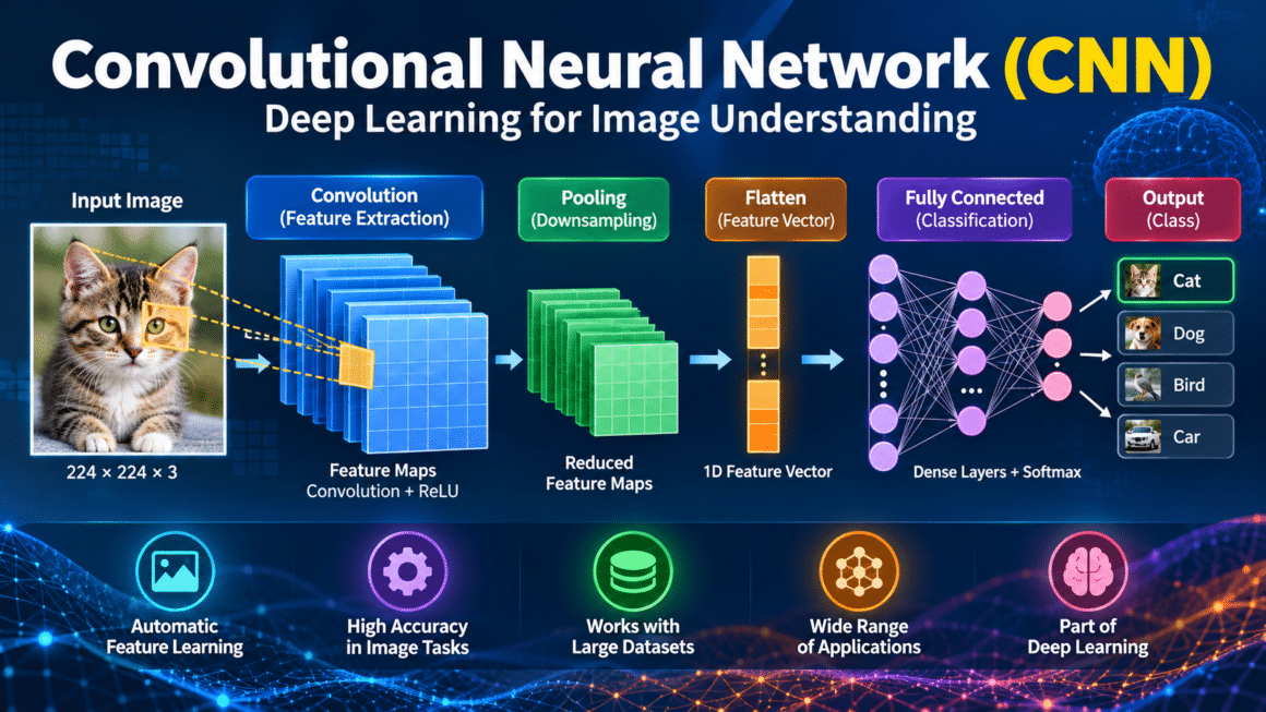
A Convolutional Neural Network (CNN) is a deep learning model designed to learn patterns from grid-like data, especially images. CNNs use learnable filters to detect local features such as edges, textures, shapes, and increasingly complex objects. By combining convolutional layers, nonlinear activation functions, pooling or other downsampling operations, and task-specific output layers, a CNN can learn useful representations directly from training examples instead of relying entirely on manually designed features.
This guide explains the Convolutional Neural Network (CNN) algorithm from its basic concepts to its mathematical operations, training procedure, worked example, flow diagram, pseudocode, advantages, limitations, and applications. It also discusses practical decisions such as data preprocessing, loss functions, backpropagation, regularization, and evaluation. Although CNNs are commonly associated with image classification, the same principles can be adapted for object detection, image segmentation, medical imaging, video analysis, audio processing, and other structured signals.
What Is a Convolutional Neural Network (CNN) Algorithm?
A Convolutional Neural Network is a neural network architecture that applies convolutional operations to learn spatial or local patterns. In a conventional fully connected network, every neuron in one layer may connect to every output of the preceding layer. For high-resolution images, this can create an enormous number of parameters. CNNs reduce this burden through local connectivity and weight sharing: each filter examines a small receptive field, and the same filter weights are reused at different positions.
For example, a CNN trained to classify photographs may first learn filters that respond to simple edges or color transitions. Deeper layers combine these responses into corners, textures, parts, and higher-level patterns. A final classification head maps the learned representation to class scores or probabilities. The network learns its filters from labeled examples by minimizing a loss function with gradient-based optimization, typically using backpropagation and an optimizer such as stochastic gradient descent or Adam.
The word “algorithm” in CNN usually refers to the complete learning pipeline rather than one isolated equation. It includes preparing the dataset, defining the architecture, performing forward propagation, calculating the loss, propagating gradients backward, updating weights, validating the model, and evaluating performance on unseen data. The exact architecture depends on the task and may include convolution, normalization, activation, pooling, residual connections, attention, or other components.
Introduction to the CNN Algorithm
Images and many other signals have meaningful local structure. Neighboring pixels are often related, and the spatial arrangement of patterns carries information. CNNs exploit this structure by applying small filters across the input. Rather than learning a separate parameter for every input-output pair, the model learns a compact collection of filters and reuses them throughout the image. This design is both computationally practical and well suited to visual pattern recognition.
Early neural-network research established the foundations for learning distributed representations, while convolutional architectures developed from research on visual processing and pattern recognition. CNNs became widely influential in computer vision after deep networks trained on large datasets and accelerated hardware achieved strong results in image classification. Modern CNN families include LeNet, AlexNet, VGG, Inception, ResNet, and MobileNet. These designs differ in depth, filter sizes, computational cost, skip connections, and efficiency, but they share the idea of learning spatial features through convolution-like operations.
A CNN typically has three broad functional stages. First, feature-extraction layers transform raw input into feature maps. Second, deeper layers combine low-level responses into more abstract representations. Third, a prediction head produces the required output, such as class probabilities, bounding boxes, or a pixel-wise segmentation map. Training adjusts the network’s parameters so that predictions align with the target labels or other training objectives.
For supervised classification, the training data consist of inputs and their corresponding labels. The model predicts a class distribution, the loss measures the difference between predictions and labels, and backpropagation calculates how each trainable parameter contributed to the error. An optimizer then adjusts the parameters. This cycle repeats over mini-batches and epochs. A validation set helps tune hyperparameters and detect overfitting, while a separate test set provides a final estimate of generalization.
Detailed CNN Algorithm with Formulas
3.1 Input representation and preprocessing
An image can be represented as a tensor X ∈ ℝH×W×C, where H is height, W is width, and C is the number of channels. A grayscale image typically has one channel, while a standard RGB image has three. Before training, images may be resized, converted to numeric tensors, and normalized. A common channel-wise normalization is:
x′ = (x − μ) / σ
where μ and σ are the mean and standard deviation estimated from the training data. Pixel values may also be scaled to a fixed range, such as [0,1]. The same preprocessing used during training must be applied consistently during validation, testing, and deployment. Augmentation such as random cropping, flipping, or mild color changes can create varied training examples and reduce overfitting, provided the transformations preserve the correct label.
3.2 Convolution operation
A convolutional layer applies learnable filters, also called kernels, to local regions of the input. For a two-dimensional input, a simplified convolution expression is:
Z(i,j,k) = bₖ + Σu=0Kh−1 Σv=0Kw−1 Σc=0C−1 W(u,v,c,k) X(i·s+u−p, j·s+v−p, c)
Here, W is the filter bank, bₖ is the bias for output channel k, Kh and Kw are kernel dimensions, s is stride, and p represents padding. Boundary indices are handled according to the selected padding rule. Deep-learning libraries often implement cross-correlation rather than mathematically flipped convolution, but the trainable operation is commonly called convolution. Each filter produces a feature map indicating where a learned pattern appears in the input.
The spatial output size for one dimension is commonly calculated as:
Output size = floor((Input size + 2P − K) / S) + 1
where P is padding, K is kernel size, and S is stride. With “same” padding and stride one, the output is often designed to preserve the input’s spatial dimensions. Larger strides reduce spatial resolution and computation. More filters create more output channels and allow the layer to represent different patterns.
3.3 Bias and activation function
The convolution output is passed through a nonlinear activation function. A widely used choice is the Rectified Linear Unit (ReLU):
ReLU(z) = max(0,z)
ReLU keeps positive responses and sets negative responses to zero. Without nonlinear activations, a stack of linear layers would remain equivalent to a single linear transformation, limiting the network’s ability to model complex patterns. Other activations include GELU, SiLU, and Leaky ReLU. The appropriate choice depends on the architecture and task.
3.4 Pooling and downsampling
Pooling reduces the spatial dimensions of feature maps. In max pooling, each local window is replaced by its maximum value:
Y(i,j,c) = max { X(i·s+u, j·s+v,c) : (u,v) ∈ window }
Average pooling replaces the maximum with the average of the window. Downsampling can reduce computation and provide some tolerance to small translations. However, aggressive pooling can discard fine spatial details, which may be harmful in tasks such as precise segmentation. Many modern networks also use strided convolutions or carefully designed feature pyramids instead of relying heavily on pooling.
3.5 Feature hierarchy and deeper layers
Multiple convolutional blocks are stacked so that later layers receive increasingly abstract feature maps. A shallow layer may respond to a simple edge, while a deeper layer may combine several responses into a texture or object part. The receptive field—the portion of the original input that can influence a feature—increases as layers are stacked and downsampling is applied. Batch normalization or other normalization layers may be inserted to stabilize training, and residual connections can help gradients pass through very deep networks.
A simplified block can be written as:
Hl = Activation(Norm(Conv(Hl−1)))
where Hl−1 is the previous feature representation and Hl is the current one. This expression is illustrative; real networks may change the order of normalization and activation or include skip connections, multiple convolutions, or attention modules.
3.6 Flattening or global pooling
For classification, the final feature maps must be transformed into a representation suitable for the output layer. One option is flattening, which reshapes all spatial features into a vector. Another is global average pooling, which averages each channel across spatial positions:
gₖ = (1 / HW) Σᵢ Σⱼ H(i,j,k)
Global average pooling often reduces the number of parameters compared with a large fully connected layer and may help reduce overfitting. The choice depends on the network design and the information the prediction head needs to preserve.
3.7 Fully connected layer and output probabilities
For a classification task with K classes, a linear output layer produces logits:
z = Wh + b
where h is the learned feature vector. The softmax function converts logits into class probabilities:
pₖ = exp(zₖ) / Σⱼ exp(zⱼ)
The predicted class is typically the class with the highest probability. Softmax probabilities are model outputs, not necessarily calibrated probabilities; calibration may be needed for applications that depend on trustworthy confidence estimates. For binary classification, a sigmoid output is also commonly used.
3.8 Loss function
The loss function quantifies how far predictions are from the target. For single-label multi-class classification, categorical cross-entropy for a one-hot target y can be expressed as:
L = −Σₖ yₖ log(pₖ)
For a batch of B examples, the average loss is:
Lbatch = (1/B) Σi=1B Lᵢ
Other tasks use different losses. Binary classification often uses binary cross-entropy; regression may use mean squared error or mean absolute error; segmentation can use pixel-wise cross-entropy, Dice loss, or combinations. The loss must match the target format and task.
3.9 Backpropagation and gradient computation
Backpropagation applies the chain rule to calculate the derivative of the loss with respect to each trainable parameter. For a parameter θ, the gradient is:
g = ∂L / ∂θ
The gradients are propagated from the output layer backward through the classifier, activation functions, pooling operations, and convolutional filters. For a convolutional layer, the gradient with respect to a filter depends on the input patches and the gradient arriving from the layer above. Modern frameworks compute these derivatives automatically, but understanding the chain-rule principle helps diagnose learning problems and select suitable architectures.
3.10 Parameter update using an optimizer
With basic stochastic gradient descent, the update for a parameter is:
θt+1 = θt − η ∇θL
where η is the learning rate. Momentum incorporates a running direction to smooth updates. Adam maintains moving averages of gradients and squared gradients, adapting the effective step size for each parameter. The learning rate, optimizer, batch size, weight decay, and schedule can strongly affect training speed and final performance. These values should be selected using validation data, not the test set.
3.11 Epochs, validation, and regularization
An epoch is one pass through the training set. Training usually processes the data in mini-batches and repeats the forward pass, loss computation, backward pass, and optimizer update for each batch. At the end of an epoch, validation metrics are measured without updating the weights. Techniques such as data augmentation, dropout, weight decay, label smoothing, and early stopping may improve generalization. Early stopping halts training when validation performance stops improving according to a defined rule.
Overfitting occurs when a model performs well on training examples but poorly on unseen data. Underfitting occurs when the model cannot learn the training patterns adequately. Learning curves, per-class metrics, confusion matrices, and validation loss help identify these problems. The final model should be evaluated on a held-out test set that was not used for model selection.
Explanation of the CNN Algorithm
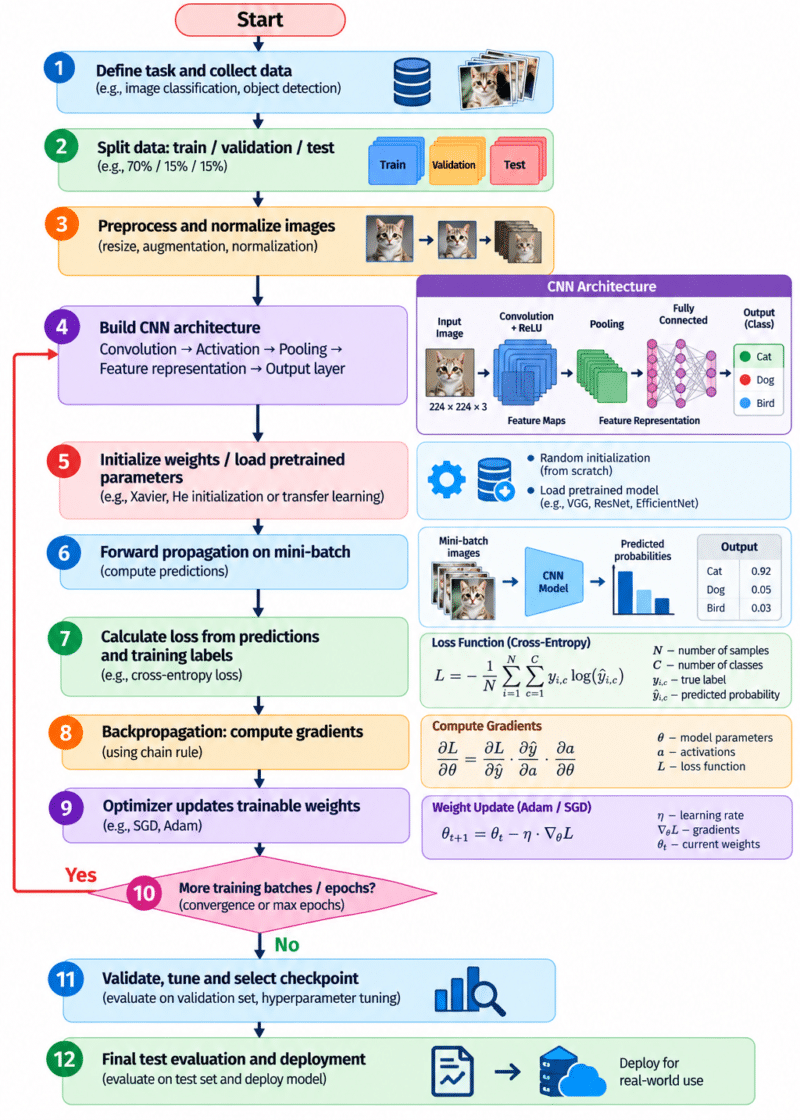
Step 1—Collect and label data. Gather representative examples for the task and verify that the labels are reliable. Split the data into training, validation, and test sets at the appropriate unit of independence. For example, in medical imaging, images from the same patient should not leak across training and test sets when patient-level generalization is being evaluated. Check class balance, image quality, duplicates, and potential data leakage before training begins.
Step 2—Preprocess the inputs. Convert images into a consistent shape and numeric format. Normalize pixel values or channels using statistics derived from the training data. Apply suitable augmentation to the training set when it reflects plausible variations. Do not apply random training augmentation to the test set unless the evaluation protocol specifically requires it. Store preprocessing settings so that inference uses the same transformations.
Step 3—Design the CNN architecture. Choose the number of convolutional blocks, filters, kernel sizes, strides, padding, activations, and downsampling operations. Select a prediction head appropriate to classification, detection, segmentation, or regression. Small datasets may benefit from transfer learning with a pretrained CNN rather than training a large network from scratch. The architecture should reflect available compute, input resolution, and latency requirements.
Step 4—Initialize the model parameters. Trainable filters and biases are initialized before learning begins. Common initialization methods, such as He initialization for ReLU-based networks or Xavier/Glorot initialization for suitable activations, aim to maintain reasonable activation and gradient scales. Biases are often initialized to zero. A pretrained model starts from learned parameters and may replace its final classification head to match the target classes.
Step 5—Perform forward propagation. Feed a mini-batch through the network. Each convolutional layer computes feature maps, activation functions introduce nonlinearity, and pooling or strided operations reduce spatial dimensions where required. Deeper blocks combine lower-level features into more abstract representations. The output head produces logits, probabilities, bounding boxes, masks, or other predictions depending on the task.
Step 6—Calculate the loss. Compare the model outputs with the training labels using the selected loss function. For multi-class image classification, cross-entropy is common. For object detection or segmentation, the loss may combine several terms for classification, localization, and mask quality. Ensure that the target encoding, output activation, and loss implementation are compatible; for example, some cross-entropy implementations expect raw logits rather than already-softmaxed probabilities.
Step 7—Backpropagate the error. Compute the gradients of the loss with respect to all trainable parameters. Backpropagation moves backward through the computational graph, applying the chain rule. Gradients indicate how parameter changes would affect the current batch’s loss. In practical implementations, automatic differentiation in frameworks such as PyTorch or TensorFlow handles these calculations.
Step 8—Update the parameters. The optimizer uses the gradients to adjust filters, biases, and other trainable parameters. The learning rate controls the size of the update. If the learning rate is too high, training may become unstable; if it is too low, convergence may be slow. Learning-rate schedules, gradient clipping, weight decay, and mixed-precision training may be useful depending on the model and hardware.
Step 9—Repeat over mini-batches and epochs. Continue processing the training data until an epoch is complete, then evaluate the model on the validation set. Track both loss and task-relevant metrics. Save checkpoints when validation performance improves and use early stopping if the model begins to overfit. Hyperparameter changes should be based on validation results, leaving the test set untouched until final evaluation.
Step 10—Evaluate and deploy. After model selection, evaluate once on the held-out test set. Report appropriate metrics, such as accuracy, precision, recall, F1-score, ROC-AUC, mean average precision, intersection over union, or regression error. Inspect errors by class and relevant subgroups. Before deployment, verify latency, memory use, input validation, robustness, and monitoring requirements. Model performance can change when real-world data differ from the training distribution.
Example: How a Convolutional Neural Network Works
Consider a simplified task of classifying small grayscale images as either a handwritten digit “0” or “1.” Each input is a 28 × 28 image with one channel. The training dataset contains images and their correct labels. The goal is for the CNN to learn the visual differences between the two digit shapes, including curves, strokes, and their spatial arrangement.
First, the image is normalized so that its pixel values are on a consistent scale. A convolutional layer applies several 3 × 3 filters. One filter may learn to respond to vertical edges, another to horizontal transitions, and another to curved patterns. These are learned during training rather than manually specified. With stride one and padding that preserves dimensions, each filter produces a 28 × 28 feature map. ReLU then keeps positive activations and removes negative values.
A 2 × 2 max-pooling layer with stride two reduces each feature map to 14 × 14. A second convolutional block may learn more complex combinations of edges and strokes, followed by another downsampling step to 7 × 7. The resulting feature maps are converted to a vector using flattening or global pooling. A final linear layer produces two logits, one for digit 0 and one for digit 1. Softmax can turn these logits into probabilities for interpretation.
Suppose the network outputs probabilities [0.20, 0.80] for an image whose true label is “1.” The model predicts class 1, and the prediction agrees with the label. If it instead outputs [0.75, 0.25], cross-entropy assigns a larger penalty because the model gives low probability to the correct class. Backpropagation calculates how the filters and classifier contributed to that error, and the optimizer updates them. Across many labeled images and training iterations, the filters gradually become more useful for separating the classes.
This example is illustrative rather than a report of measured results. Actual accuracy depends on dataset quality, network design, training procedure, and evaluation protocol. A robust experiment should compare a CNN with suitable baselines, use a held-out test set, and report multiple metrics when class imbalance or error costs make accuracy alone insufficient.
The following flowchart summarizes the training pipeline from dataset preparation through prediction and final evaluation.
Pseudocode for the CNN Algorithm
Input:
    Training data D_train
    Validation data D_val
    CNN architecture f_theta
    Loss function L
    Optimizer Opt
    Number of epochs E
    Batch size B

Initialize model parameters theta
best_validation_score = initial value
best_checkpoint = none

for epoch = 1 to E:
    Set model to training mode
    Shuffle D_train

    for each mini-batch (X, y) in D_train of size B:
        X = preprocess_and_augment(X)

        # Forward propagation
        predictions = f_theta(X)

        # Compute objective
        loss = L(predictions, y)

        # Backpropagation
        Opt.zero_grad()
        loss.backward()

        # Parameter update
        Opt.step()

    Set model to evaluation mode
    validation_metrics = evaluate(f_theta, D_val)

    if validation score improves:
        best_checkpoint = save(theta)
        best_validation_score = validation score

    if early-stopping criterion is satisfied:
        break

Restore best_checkpoint
test_metrics = evaluate(f_theta, held-out test data)

Return trained model and test_metrics
The pseudocode describes a standard supervised CNN training loop. Real code must implement the architecture, data loader, correct loss/output pairing, device placement, optimizer configuration, metric calculations, and checkpoint handling. During validation and testing, gradients should normally be disabled and training-only augmentation should not be applied.
Advantages and Disadvantages of the CNN Algorithm
Advantages
- Automatic feature learning: CNNs learn useful filters from data and reduce the need for handcrafted image features.
- Local connectivity: Filters focus on local neighborhoods, which is well suited to spatially structured inputs.
- Parameter sharing: Reusing the same filter across positions can dramatically reduce parameter count compared with a fully connected layer over raw pixels.
- Hierarchical representations: Deeper layers can combine simple patterns into complex features.
- Strong performance in visual tasks: CNNs are effective for image classification, detection, segmentation, and many related applications.
- Transfer learning: Pretrained networks can provide useful starting points, especially when labeled data are limited.
- Hardware and software support: Common deep-learning frameworks and GPUs support efficient convolution operations.
Disadvantages
- Data requirements: Training a high-capacity CNN from scratch may require many representative labeled examples.
- Computational cost: Deep networks can demand substantial GPU memory, processing time, and energy.
- Hyperparameter sensitivity: Performance depends on architecture, learning rate, batch size, regularization, preprocessing, and training duration.
- Limited built-in global context: Standard convolutions focus on local neighborhoods; capturing long-range relationships may require deeper layers or additional mechanisms.
- Potential overfitting: A model can memorize training patterns, particularly with small or biased datasets.
- Interpretability challenges: It may be difficult to explain why a CNN made a specific prediction, although visualization and attribution methods can provide partial insight.
- Distribution shift and bias: A model may perform poorly on images from different devices, environments, populations, or acquisition conditions.
- Spatial detail can be lost: Pooling and downsampling can remove fine-grained information needed for precise localization.
These limitations can be addressed partly through careful data collection, transfer learning, augmentation, regularization, efficient architectures, explainability tools, and independent testing. No single architecture is optimal for every task. CNNs should be compared with relevant alternatives under a consistent evaluation protocol.
Applications of the Convolutional Neural Network (CNN) Algorithm
Image classification: CNNs assign images to categories, such as identifying animals, plant species, manufactured products, or document types. The model learns discriminative patterns from labeled examples and returns class scores or probabilities.
Object detection: Detection systems identify objects and estimate their locations using bounding boxes or related representations. CNN backbones are used in many detection architectures to extract features for people, vehicles, products, defects, and other objects.
Image segmentation: Semantic segmentation assigns a class to each pixel, while instance segmentation separates individual object instances. CNN-based encoder-decoder architectures are widely used in medical scans, satellite imagery, agriculture, and industrial inspection.
Medical imaging: CNNs can assist with image classification, lesion localization, organ segmentation, and analysis of radiographs, CT, MRI, ultrasound, and pathology images. Clinical use requires rigorous validation, representative datasets, privacy protection, human oversight, and evaluation across institutions and patient groups.
Autonomous driving and intelligent transportation: Vision systems use CNN-based features to detect lanes, traffic signs, pedestrians, vehicles, and road hazards. Safety-critical applications require testing across weather, lighting, camera, and road conditions, as well as robust system-level safeguards.
Industrial quality control: CNNs can detect scratches, cracks, surface defects, assembly errors, or abnormal product patterns. They can help automate visual inspection, but performance depends on the diversity of defect examples, camera setup, and the cost of false positives and false negatives.
Agriculture and environmental monitoring: CNNs can classify plant diseases, identify weeds, estimate crop conditions, and analyze aerial or satellite images. These models can support monitoring at scale, but should be tested across seasons, locations, species, and imaging devices.
Document and character recognition: CNNs can extract visual features for handwritten digit recognition, optical character recognition pipelines, document layout analysis, and symbol recognition. In many modern systems, CNN features are combined with sequence models or attention-based architectures.
Video analytics: CNNs can extract frame-level spatial features for action recognition, event detection, surveillance analytics, and sports analysis. Temporal modeling is often added through 3D convolutions, recurrent layers, temporal convolutions, or transformer components to represent motion and changes over time.
Audio and time-series processing: CNNs can operate on spectrograms or other time-frequency representations for speech, sound-event recognition, and music analysis. One-dimensional convolutions can also learn local temporal patterns in sensor data, industrial signals, and physiological measurements.
Remote sensing and geospatial analysis: CNNs can classify land cover, map buildings, detect changes, and analyze satellite or drone imagery. Spatial resolution, geographic variation, seasonal effects, and annotation quality are important considerations when evaluating generalization.
Across these applications, the same general learning loop is used, but the data representation, output head, loss function, and evaluation metrics must be tailored to the task. A successful deployment also needs monitoring for changing input distributions, data quality issues, latency constraints, and model degradation.
Conclusion
The Convolutional Neural Network is a foundational deep learning algorithm for extracting patterns from images and other structured data. Convolutional filters learn local features, activation functions add nonlinearity, pooling or strided operations control spatial resolution, and deeper layers form increasingly abstract representations. A task-specific output layer produces predictions, while a loss function and backpropagation guide parameter updates during training.
A reliable CNN workflow requires more than choosing layers. It begins with careful dataset preparation, sound train-validation-test separation, appropriate preprocessing, and an architecture matched to the task. Training should track validation performance, use regularization where needed, and preserve the best checkpoint. Final evaluation should report relevant metrics and examine errors, subgroup performance, robustness, and deployment cost.
CNNs have enabled advances in image classification, detection, segmentation, medical imaging, industrial inspection, agriculture, video analytics, and many other fields. However, they can be data-intensive, computationally expensive, and vulnerable to overfitting or distribution shift. Researchers and practitioners should compare them with suitable baselines, document experiments clearly, and validate models in the conditions where they will be used. When developed and evaluated carefully, CNNs provide a flexible and powerful framework for data-driven pattern recognition.
Frequently Asked Questions (FAQs)
1. What does CNN stand for?
CNN stands for Convolutional Neural Network. It is a deep learning architecture that uses learnable convolutional filters to extract local patterns from images and other structured inputs.
2. How does a CNN learn image features?
During training, the network predicts outputs, calculates a loss, computes gradients through backpropagation, and updates its filters with an optimizer. Repeated updates help filters become useful for the target task.
3. What is the role of a convolutional layer?
A convolutional layer applies shared learnable filters to local regions of the input. Each filter produces a feature map that responds to patterns such as edges, textures, or more complex structures.
4. Why are activation functions used in CNNs?
Activation functions introduce nonlinearity. Without nonlinear activations, a stack of linear operations would still behave like a single linear transformation and would be unable to represent many complex patterns.
5. What is the difference between convolution and pooling?
Convolution applies learnable filters to extract features. Pooling reduces spatial dimensions using a fixed aggregation rule, such as taking the maximum or average within each window.
6. Can CNNs be trained with small datasets?
Yes, but training from scratch may overfit. Transfer learning, data augmentation, regularization, careful validation, and collecting more representative data can improve results when datasets are limited.
7. Which metrics are used to evaluate a CNN?
Metrics depend on the task. Classification may use accuracy, precision, recall, F1-score, and ROC-AUC; object detection may use mean average precision; segmentation may use intersection over union or Dice score; regression may use MAE or RMSE.
References
- LeCun, Y., Bottou, L., Bengio, Y., & Haffner, P. (1998). “Gradient-Based Learning Applied to Document Recognition.” Proceedings of the IEEE, 86(11), 2278–2324. https://doi.org/10.1109/5.726791
- Krizhevsky, A., Sutskever, I., & Hinton, G. E. (2012). “ImageNet Classification with Deep Convolutional Neural Networks.” Advances in Neural Information Processing Systems, 25. NeurIPS paper
- Simonyan, K., & Zisserman, A. (2015). “Very Deep Convolutional Networks for Large-Scale Image Recognition.” International Conference on Learning Representations (ICLR). arXiv:1409.1556
- He, K., Zhang, X., Ren, S., & Sun, J. (2016). “Deep Residual Learning for Image Recognition.” Proceedings of the IEEE Conference on Computer Vision and Pattern Recognition (CVPR), 770–778. https://doi.org/10.1109/CVPR.2016.90
- Goodfellow, I., Bengio, Y., & Courville, A. (2016). Deep Learning. MIT Press. Online book
Further Learning
- TensorFlow: Convolutional Neural Network tutorial — practical image-classification example.
- PyTorch: Training a classifier on CIFAR-10 — implementation-oriented tutorial.
- Deep Learning textbook — foundational material on neural networks and optimization.
- Very Deep Convolutional Networks (VGG) — research paper on deeper CNN architectures.
- Deep Residual Learning (ResNet) — research paper on residual connections for training deep networks.