

Cat Swarm Optimization (CSO) is a population-based metaheuristic optimization algorithm inspired by the natural behaviors of cats, especially their tendency to spend much of their time observing their surroundings and occasionally moving quickly to pursue a target. In optimization, each cat represents a candidate solution. The algorithm combines two complementary search behaviors—seeking mode, which explores nearby alternatives, and tracing mode, which moves a candidate toward a promising solution. This combination helps CSO search complex solution spaces where conventional gradient-based methods may be difficult to apply.
This tutorial introduces the principles, mathematical model, step-by-step procedure, worked example, pseudocode, strengths, limitations, applications, and references for Cat Swarm Optimization. It also explains practical choices such as population size, seeking memory pool, mutation range, and the mixture ratio. CSO is a stochastic optimization method: its results can vary between runs, so implementations should use reproducible random seeds during experiments and evaluate performance over multiple independent runs.
What Is Cat Swarm Optimization (CSO) Algorithm?
Cat Swarm Optimization is a swarm-intelligence algorithm introduced by Shu-Chuan Chu and Pei-Wei Tsai in 2007. It models two stylized behaviors. In seeking mode, a cat remains relatively still while examining possible changes to its current position; this resembles local exploration. In tracing mode, the cat moves in the direction of a velocity vector toward a promising position; this resembles directed exploitation. A control parameter called the mixture ratio (MR) determines the proportion of cats assigned to tracing mode, while the remaining cats perform seeking behavior.
For a problem with D decision variables, the position of cat i can be represented as a vector xᵢ = (xᵢ₁, xᵢ₂, …, xᵢD). A cat may also have a velocity vector vᵢ, which controls how its position changes in tracing mode. A fitness function evaluates each position and indicates how good that candidate solution is. For minimization, smaller fitness values are better; for maximization, larger values are better. The algorithm maintains the best solution found so far and iteratively updates the population until a stopping condition is met.
CSO is not a biological simulation intended to reproduce every aspect of feline behavior. Instead, it is an abstract optimization framework that borrows the seeking/tracing analogy to balance exploration and exploitation. Like other metaheuristics, it does not guarantee the global optimum for every problem, but it can be useful when the objective function is nonlinear, discontinuous, noisy, non-differentiable, or expensive to model analytically.
Introduction to Cat Swarm Optimization (CSO)
Many optimization tasks require finding a good combination of variables from a large search space. Examples include selecting features for a machine-learning model, tuning hyperparameters, scheduling jobs, routing packets, configuring engineering designs, and allocating resources. Exhaustive search becomes impractical as the number of possible solutions increases. Gradient-based algorithms may also be unsuitable when derivatives are unavailable or the search space contains discrete decisions. Population-based metaheuristics address these challenges by maintaining several candidate solutions and improving them through stochastic search.
CSO belongs to the broader family of swarm-intelligence and nature-inspired optimization methods. Its population is called a swarm, and each member is called a cat. Each cat has a position, a fitness value, and a mode assignment. Tracing cats update their velocities and move through the search space; seeking cats generate and compare nearby candidate positions. The algorithm periodically evaluates all new positions and updates the global best candidate.
The main design idea is that exploration and exploitation should occur together. Exploration helps the algorithm visit different regions and avoid becoming trapped too early in a poor local optimum. Exploitation concentrates search around promising regions to refine a solution. If every cat only explored randomly, convergence could be slow. If every cat only followed the current best, the population could lose diversity and converge prematurely. The seeking/tracing balance is intended to reduce this tension.
CSO has several variants, including binary CSO for discrete decisions, multi-objective CSO for competing objectives, and hybrid CSO methods that combine it with local search or other optimizers. These variants modify the representation or update rules to fit the problem. Therefore, the exact equations and parameter meanings should always be checked in the particular CSO variant being implemented.
Detailed Cat Swarm Optimization Algorithm
3.1 Define the optimization problem
First, express the task as an objective function:
Minimize: f(x), subject to Lⱼ ≤ xⱼ ≤ Uⱼ, for j = 1, 2, …, D.
Here, x is a candidate vector, f(x) is the objective or fitness function, and Lⱼ and Uⱼ are the lower and upper bounds of variable j. For maximization, the comparison direction is reversed, or the objective can be transformed into an equivalent minimization problem. Constraints can be handled with repair rules, feasibility-first comparison, or penalty functions.
3.2 Initialize the swarm
Choose a population size N. Randomly initialize each cat’s position within the allowed bounds. For continuous variables, a common initialization rule is:
xᵢⱼ = Lⱼ + rᵢⱼ (Uⱼ − Lⱼ)
where rᵢⱼ is drawn independently from a uniform distribution U(0,1). Initialize each velocity, often to zero or to a small random value within a permitted range. Evaluate every initial position and record the best position as the global best g. Initialization should cover the search space reasonably well; stratified or problem-informed initialization may be used where appropriate.
3.3 Assign seeking and tracing modes
The mixture ratio MR controls how many cats trace and how many seek. Conceptually, MR is the fraction assigned to tracing mode. Implementations commonly assign modes randomly or use a controlled count close to MR × N. The remaining cats are assigned seeking mode. MR is generally represented between 0 and 1, although some published implementations express it as a percentage. Keep the convention consistent throughout the code.
3.4 Seeking mode: local exploration
Seeking mode generates several candidate copies or neighbors around a cat’s current position. Important parameters include the seeking memory pool (SMP), the seeking range of selected dimensions (SRD), the counts of dimension to change (CDC), and a self-position consideration (SPC) option. SMP determines how many candidate positions are considered. CDC controls the fraction or number of dimensions selected for modification. SRD controls the relative magnitude of a change. SPC specifies whether the original position is included among the candidates.
A simplified continuous perturbation for a selected dimension can be written as:
x′ᵢⱼ = xᵢⱼ + ρ × SRD × (Uⱼ − Lⱼ)
where ρ is a random value, often sampled from a symmetric interval such as [−1,1]. This is an illustrative neighbor-generation rule; exact implementations differ in how dimensions are selected, how perturbations are sampled, and how the original position is included. After generating candidates, repair any variables that fall outside their bounds, evaluate their fitness, and select one candidate. A common probability rule assigns greater selection probability to better candidates. For minimization, one possible normalized rule is:
Pₖ = (fₘₐₓ − fₖ) / Σₗ(fₘₐₓ − fₗ)
where fₘₐₓ is the worst fitness among the candidates. This rule requires care when all fitness values are equal; in that case, select uniformly at random or use a small numerical safeguard. If the denominator is nonzero, candidates with lower objective values receive higher probability. For maximization, reverse the normalization appropriately. An implementation may instead use rank-based probabilities to avoid scaling problems.
3.5 Tracing mode: directed movement
Tracing mode updates a cat’s velocity and position using its current position and the best-known position. A common particle-swarm-like update is:
vᵢⱼ(t+1) = vᵢⱼ(t) + rⱼ × c × [gⱼ − xᵢⱼ(t)]
xᵢⱼ(t+1) = xᵢⱼ(t) + vᵢⱼ(t+1)
Here, vᵢⱼ is the velocity of cat i in dimension j, gⱼ is the corresponding coordinate of the global-best position, rⱼ is a random number in [0,1], and c is an acceleration coefficient. Some CSO descriptions use a velocity update without an explicit inertia term, while variants may add an inertia weight or other coefficients. If velocity becomes too large, clamp it to a maximum magnitude Vmax or use another velocity-control strategy.
After moving, enforce variable bounds, evaluate the new position, and update the cat’s current state. If the new fitness improves the best-known fitness, update the global best. In constrained problems, a feasible solution may be preferred over an infeasible one even when its raw objective value is worse. The comparison policy should reflect the task’s actual constraints.
3.6 Fitness evaluation and global-best update
Fitness evaluation connects the general optimizer to the application. For feature selection, fitness might combine prediction error with a penalty for selecting too many features. For engineering design, it could represent cost, weight, energy use, or a weighted combination of objectives. The global-best update is:
g(t+1) = xᵢ(t+1) if f(xᵢ(t+1)) < f(g(t)) for a minimization problem; otherwise, retain g(t).
Store the best fitness and, if useful, the history of best fitness values. This history supports convergence plots and helps determine whether the algorithm is improving or stagnating. For stochastic or noisy objectives, repeated evaluation or statistical comparisons may be necessary.
3.7 Boundary handling and constraints
A movement or perturbation can produce a value outside the allowed range. A simple clipping repair is:
xᵢⱼ ← min(Uⱼ, max(Lⱼ, xᵢⱼ))
Clipping is straightforward but can accumulate candidates at the boundaries. Alternatives include reflecting the position back into the range, resampling the invalid coordinate, or using problem-specific repair. For constrained optimization, a penalty formulation may be used:
F(x) = f(x) + λ Σₘ max(0, hₘ(x))²
where hₘ(x) ≤ 0 denotes an inequality constraint and λ is a penalty coefficient. Equality constraints need their own violation term, such as a squared residual. Penalties should be scaled carefully because an excessively large or small penalty can distort the search.
3.8 Termination
Repeat mode assignment, seeking/tracing updates, evaluation, and best-solution tracking until a stopping criterion is reached. Common criteria are a maximum number of iterations, a maximum number of objective evaluations, a time budget, or a tolerance indicating that improvement has become very small for several iterations. The final output is the best candidate and its fitness, together with optional convergence history and runtime statistics.
Step-by-Step Explanation of CSO
Step 1—Represent the problem. Identify the variables that must be optimized, their allowed ranges, the objective to minimize or maximize, and any constraints. Decide whether variables are continuous, integer, binary, or mixed. This decision determines how positions are encoded and how seeking-mode modifications are generated. A clear representation is essential because CSO only searches the representation it is given.
Step 2—Choose parameters and initialize cats. Select a population size, maximum iterations, mixture ratio, seeking memory pool, seeking range, counts of dimensions to change, tracing coefficient, and any velocity limit. Randomly generate the starting positions and initialize velocities. Evaluate each cat and identify the best initial solution. Parameter values are problem-dependent; begin with reasonable values, then tune them through repeated experiments rather than assuming a single setting works for every dataset.
Step 3—Assign each cat a search behavior. For each iteration, decide which cats will trace and which will seek. Tracing is intended to exploit a promising region by moving toward the global best. Seeking is intended to explore nearby alternatives and retain opportunities to discover better regions. The mixture ratio governs the balance, so an extremely high tracing fraction may reduce diversity, while an extremely low tracing fraction may make convergence slow.
Step 4—Generate seeking candidates. For every cat in seeking mode, create a pool of nearby candidate positions. Select the dimensions to change according to CDC and modify them according to SRD or the implementation’s chosen perturbation rule. Depending on SPC, include or exclude the cat’s current position. Repair invalid values, calculate the fitness of each candidate, and choose one candidate with a probability rule favoring better fitness. This stage allows local experimentation without requiring gradients.
Step 5—Move tracing cats. For each cat in tracing mode, calculate a new velocity based on its previous velocity and the difference between the global-best position and its current position. Use the resulting velocity to update its position. Apply any velocity limit and boundary repair. This movement encourages the population to concentrate on areas that have already produced good solutions, while random factors preserve some variation in movement.
Step 6—Evaluate and update the best solution. Calculate the objective value of every updated cat. Compare each new candidate with the best solution found so far. If it is better and satisfies the chosen feasibility policy, store it as the new global best. Keep the best candidate independently of the current population so that a later movement does not accidentally lose the best result already discovered.
Step 7—Check the stopping rule and report results. If the iteration or evaluation budget has not been exhausted, return to mode assignment and continue searching. Otherwise, report the best solution, objective value, number of evaluations, runtime, and relevant constraints. Because CSO is stochastic, run it several times with different seeds and report summary statistics such as mean, standard deviation, median, and best result. Compare it with appropriate baselines under the same evaluation budget.
Example: How Cat Swarm Optimization Works
Consider a simple one-dimensional minimization problem: minimize f(x) = (x − 3)², subject to −5 ≤ x ≤ 5. The true optimum is x = 3, where the objective value is zero. This example illustrates the mechanics rather than prescribing a universal parameter setting. Suppose the swarm begins with three cats at x = −2, x = 0, and x = 4. Their fitness values are respectively 25, 9, and 1. Therefore, the initial global best is x = 4, with fitness 1.
Assume the first cat is assigned seeking mode. It generates candidate neighbors around x = −2, perhaps x = −1 and x = 1, while also considering its original position if SPC is enabled. The fitness values are 16 and 4 for those two neighbors, compared with 25 for the original point. The candidate at x = 1 is the best among these illustrative choices, so the cat may select it. The population has now explored a better local position, but x = 4 remains the global best because its fitness is still lower than 4.
Next, suppose the second cat at x = 0 is assigned tracing mode. For illustration, let its velocity initially be zero, the random factor r = 0.5, and acceleration coefficient c = 1. Using v(t+1) = v(t) + r c (g − x), its new velocity is 0 + 0.5(4 − 0) = 2. The new position is x = 0 + 2 = 2, and its fitness is (2 − 3)² = 1. The result ties the current best fitness. If another seeking candidate or tracing step reaches x = 3, the fitness becomes zero and the global best is updated to x = 3.
This small example demonstrates the complementary roles of the two modes. Seeking evaluates nearby alternatives and can improve a cat’s current location. Tracing uses the best-known location to direct movement through the search space. In a real multidimensional problem, the position is a vector, candidate generation can affect selected dimensions, and many cats are updated over many iterations. The optimum is not guaranteed to be found in every run, so the example should be interpreted as an explanation of the update logic, not a performance guarantee.
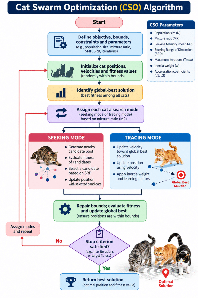
Digital Diagram for Cat Swarm Optimization (CSO)
The following workflow diagram summarizes the main stages of CSO from problem definition through initialization, mode assignment, the two search behaviors, fitness evaluation, global-best updating, and termination.
Pseudocode for Cat Swarm Optimization
Input: objective f(x), bounds L and U, population N,
       maximum iterations T, mixture ratio MR,
       seeking parameters SMP, SRD, CDC, SPC,
       tracing coefficient c and velocity limit Vmax

Initialize positions x[i] within [L, U]
Initialize velocities v[i]
Evaluate fitness f(x[i]) for all cats
g = best initial position

for t = 1 to T:
    Assign each cat to seeking or tracing mode
    according to mixture ratio MR

    for each cat i:
        if cat i is in SEEKING mode:
            Create SMP candidate positions near x[i]
            Select dimensions to modify using CDC
            Apply perturbations controlled by SRD
            Include current position according to SPC
            Repair candidates that violate bounds
            Evaluate candidate fitness values
            Select a candidate, favoring better fitness
            x[i] = selected candidate

        else:  # TRACING mode
            for each dimension j:
                v[i,j] = v[i,j] + random(0,1)
                         * c * (g[j] - x[i,j])
                v[i,j] = clamp(v[i,j], -Vmax, Vmax)
                x[i,j] = x[i,j] + v[i,j]
            Repair x[i] to satisfy bounds

        Evaluate f(x[i])
        if x[i] is better than g under the
           objective and constraint policy:
            g = x[i]

    Record best fitness and other diagnostics
    if another stopping criterion is satisfied:
        break

return g and f(g)
This pseudocode expresses the general workflow. A production implementation must define the precise candidate-copy rules, the sampling distribution, how equal fitness values are handled, constraint repair, and the exact interpretation of MR. For reproducibility, record all parameter values and the random seed.
Advantages and Disadvantages of CSO
Advantages
- Balances exploration and exploitation: Seeking mode explores local alternatives while tracing mode directs search toward good solutions.
- Does not require gradients: It can optimize objectives for which derivatives are unavailable, unreliable, or expensive.
- Flexible objective functions: With suitable encoding and evaluation, CSO can be adapted to engineering, scheduling, feature selection, and machine-learning tasks.
- Population-based search: Multiple candidates are maintained, which can help explore different regions instead of relying on a single starting point.
- Adaptable framework: Binary, multi-objective, hybrid, and problem-specific variants can be designed for different optimization structures.
- Conceptually understandable: The seeking/tracing metaphor provides an intuitive way to explain local candidate exploration and directed movement.
Disadvantages
- No guarantee of a global optimum: CSO is stochastic and may converge to a local or suboptimal solution.
- Parameter sensitivity: Performance can depend on population size, MR, SMP, SRD, CDC, tracing coefficient, and velocity limits.
- Computational cost: Seeking mode may evaluate multiple candidates per cat, increasing the number of objective-function calls.
- Premature convergence: If tracing dominates or population diversity becomes low, cats may cluster around a suboptimal region.
- Representation challenges: Discrete, binary, mixed-variable, and heavily constrained problems require careful encoding and repair rules.
- Implementation differences: Variants may define parameters and update equations differently, making results difficult to compare unless methods are described precisely.
- Stochastic variability: A single run may be misleading. Multiple runs and statistical reporting are needed for reliable evaluation.
To use CSO responsibly, establish a baseline, tune parameters systematically, track objective evaluations, preserve the best solution, and test multiple random seeds. Report not only the best result but also typical performance and computational cost. For a fair comparison, use the same data splits, stopping budgets, constraints, and evaluation procedures for competing algorithms.
Applications of Cat Swarm Optimization
Feature selection and machine learning: CSO can search for a subset of informative features while balancing predictive performance and subset size. A sample minimization objective is F(S) = α(1 − Accuracy(S)) + β|S|/D, where S is the selected feature set, D is the total number of features, and α and β control the trade-off. Binary CSO or a discrete encoding is usually needed because a feature is either selected or not selected. Evaluation should use training/validation data carefully to avoid leakage.
Neural-network and model hyperparameter tuning: A cat can encode learning rate, regularization strength, number of units, batch size, or other tunable parameters. Since some hyperparameters are discrete and others continuous, a mixed representation may be necessary. The fitness value can be validation loss or another metric, and the evaluation budget should account for the cost of training each model.
Engineering design and parameter estimation: CSO can optimize design dimensions, controller parameters, material choices, or model coefficients when the objective is nonlinear or simulated. Each candidate may require a numerical simulation, so the number of fitness evaluations is an important cost measure. Constraints such as stress limits, stability, or manufacturing tolerances must be enforced.
Network routing and communication systems: CSO variants can search routing configurations, channel assignments, or resource-allocation decisions. Fitness may combine end-to-end delay, energy use, packet delivery ratio, throughput, and routing overhead. Because these metrics can have different scales and conflicting objectives, normalization and explicit weighting are important. Dynamic networks may require frequent re-optimization and fast stopping criteria.
Scheduling and resource allocation: In job scheduling, cloud resource allocation, and task assignment, a candidate encodes an assignment or sequence. Objectives can include makespan, waiting time, energy use, and operating cost. Since ordinary continuous perturbations do not directly produce valid schedules, specialized swap, insertion, or repair operators are often required.
Image processing and signal processing: CSO can tune segmentation thresholds, filter coefficients, denoising parameters, or feature extraction settings. Fitness can measure reconstruction error, signal-to-noise ratio, or segmentation quality. If the evaluation is noisy or multiple objectives matter, repeated testing or a multi-objective variant may be appropriate.
Energy and power systems: Potential tasks include economic dispatch, renewable-energy scheduling, parameter tuning, and battery or microgrid operation. Such problems often have operational constraints and changing demand. A CSO-based solution must be assessed for feasibility, stability, robustness, and performance under realistic scenarios—not only on a simplified benchmark.
Data mining and clustering: CSO can optimize cluster centers, clustering parameters, or combinations of features. For clustering, fitness may be based on within-cluster dispersion or a validity index, though the chosen metric can bias the resulting structure. The algorithm should be compared with standard clustering baselines and assessed across several initializations.
These are potential application areas, not claims that CSO is always the best method. Suitability depends on the objective, encoding, constraints, evaluation cost, and quality of the baseline methods. A good study should explain why CSO is appropriate and report enough detail for another researcher to reproduce the experiment.
Conclusion
Cat Swarm Optimization is a nature-inspired, population-based metaheuristic that combines seeking and tracing behaviors to explore a search space and improve candidate solutions. Seeking mode generates and evaluates nearby alternatives, while tracing mode updates movement toward the best-known solution. A typical CSO workflow defines the objective, initializes the swarm, assigns modes, updates positions, evaluates fitness, maintains the global best, and stops when a budget or convergence criterion is met.
The algorithm is attractive because it does not require gradient information and can be adapted to many optimization tasks. However, its effectiveness depends on parameter choices, the representation of the problem, boundary and constraint handling, and the computational cost of fitness evaluation. It does not guarantee a global optimum, and different CSO variants may use different update details. Researchers should therefore document the variant, conduct repeated runs, compare against suitable baselines, and report both solution quality and computational effort. With careful design and transparent evaluation, CSO can be a useful member of an optimization toolkit rather than a universal replacement for other methods.
Frequently Asked Questions (FAQs)
1. What does CSO stand for?
CSO stands for Cat Swarm Optimization. It is a population-based metaheuristic inspired by two abstract behaviors—seeking and tracing—to search for good solutions to optimization problems.
2. Who introduced the Cat Swarm Optimization algorithm?
Cat Swarm Optimization was introduced by Shu-Chuan Chu and Pei-Wei Tsai in a 2007 publication. See the original paper listed in the references for the foundational formulation.
3. What is the difference between seeking mode and tracing mode?
Seeking mode generates and compares nearby candidate positions to explore alternatives. Tracing mode updates a cat’s velocity and position toward the current global-best solution, emphasizing directed search.
4. What is the mixture ratio in CSO?
The mixture ratio (MR) controls the proportion of cats assigned to tracing mode; the remaining cats use seeking mode. Its best value depends on the problem and should be tested empirically.
5. Does CSO always find the global optimum?
No. CSO is stochastic and does not guarantee a global optimum for arbitrary problems. Multiple independent runs, suitable stopping criteria, and comparisons with baseline methods help assess reliability.
6. Can CSO be used for feature selection?
Yes. A binary or discrete CSO variant can represent each feature as selected or not selected. The fitness function can balance validation performance against the number of selected features.
7. How is CSO performance evaluated?
Evaluate the objective value and feasibility, and also report runtime or objective-function evaluations. For stochastic algorithms, run several seeds and summarize mean, standard deviation, median, and best performance. Compare methods using the same experimental budget.
References and Further Reading
- Chu, S.-C., Tsai, P.-W. (2007). “Computational Intelligence Based on the Behavior of Cats.” International Journal of Innovative Computing, Information and Control, 3(1), 163–173. Journal issue and article information.
- Chu, S.-C., Tsai, P.-W., Pan, J.-S. (2006). “Cat Swarm Optimization.” In Proceedings of the 9th Pacific Rim International Conference on Artificial Intelligence (PRICAI 2006). Springer. SpringerLink. Search the title in the publisher catalogue for bibliographic details.
- Yang, X.-S. (2014). Nature-Inspired Optimization Algorithms. Elsevier. Publisher book page.
- Talbi, E.-G. (2009). Metaheuristics: From Design to Implementation. Wiley. Wiley publisher website.
- Particle Swarm Optimization overview, useful for understanding the velocity-based movement that appears in many tracing-mode formulations: Particle Swarm Optimization research resources.
External Resources
- ScienceDirect Topics: Metaheuristic optimization — background on metaheuristic methods.
- SpringerLink — search for peer-reviewed books and papers on swarm intelligence and CSO.
- Nature-Inspired Optimization Algorithms — broader context for nature-inspired optimization.
- Particle Swarm Optimization research resources — background on swarm-based search and velocity updates.