What is Random Forest?

Random Forest is an ensemble learning method for classification and regression that builds a collection (a “forest”) of decision trees and combines their predictions to produce a single, more robust output. For classification it uses majority voting across trees; for regression it averages the predictions. Random Forest reduces variance compared to single decision trees, improves generalization, and is relatively robust to overfitting and noise.

At its core, Random Forest relies on two ideas:

1. Bagging (Bootstrap Aggregating): Train each tree on a random bootstrap sample of the data so each tree sees a slightly different dataset.
2. Random feature selection: When splitting a node, a tree considers only a random subset of features rather than all features. This decorrelates the trees and improves diversity in the ensemble.

Introduction to Random Forest

Decision trees are intuitive and powerful but tend to overfit: they can capture noise and high variance in training data. Ensemble methods address this by combining multiple models. Random Forest is a bagging-based ensemble that adds additional randomness in feature selection.

Why Random Forest?

• Works well out-of-the-box on tabular data.
• Handles classification and regression.
• Can handle large numbers of features and examples.
• Provides feature importance measures.
• Robust to outliers and non-linear relationships.
• Requires limited hyperparameter tuning for usable performance.

Key hyperparameters include number of trees (n_estimators), maximum depth of trees (max_depth), number of features considered at each split (m_try / max_features), and minimum samples required to split a node (min_{samples_split}).

Detailed Random Forest Algorithm

Below are a concise but formal description and the math behind the main steps.

Notation

• Dataset: D={(xi,yi)}_i=1^N​ where x_i∈R^p and y_i​ is target (class label for classification, real value for regression).
• Number of trees: T.
• Each tree t trained on bootstrap sample D_t​ (sampled with replacement from D).
• For classification with K classes, predicted class probabilities by tree t at input x: P^t(y=k∣x).
• For regression, tree t’s prediction: f^t(x).

Step 1 — Bootstrap sampling (bagging)

For each tree t∈{1,…,T}:

• Create bootstrap dataset D_t​ by sampling N examples uniformly with replacement from D.
• On average, each D_t​ contains about (1−1/e)≈63.2% of unique examples (others are duplicates); the remaining ~36.8% are Out-Of-Bag (OOB) for that tree.

Step 2 — Growing a decision tree with random feature selection

Grow an unpruned decision tree on D_t​ with the following splitting rule:

At a node m with data D_m​, select a subset of features F_m of size m_try (commonly sqrt(p)​ for classification and p/3 for regression), sampled without replacement from the full p features. Consider all splits on features in Fm​ and choose the split that optimizes the impurity criterion.

Impurity criteria:

• Gini impurity (classification):

For node m with class probabilities p_mk for class k:

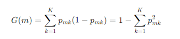
A split that partitions D_m​ into left D_L​ and right D_R produces impurity decrease:

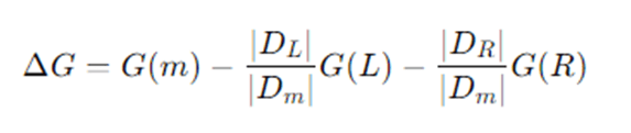
Choose the split that maximizes ΔG.

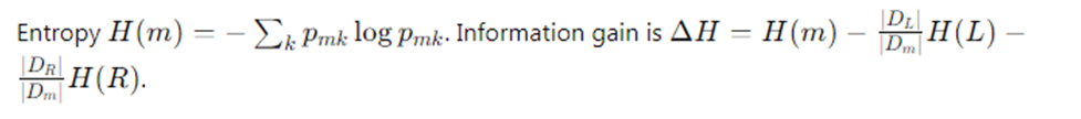
• Entropy / Information Gain (classification)

• Mean Squared Error (regression):

For regression, impurity at node m is usually variance:

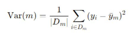
The reduction in variance is used to choose splits.

Grow each tree until a stopping criterion (max depth, minimum samples per leaf) or until nodes are pure.

Step 3 — Tree prediction

• Classification: Each tree t outputs class probabilities P^t(y=k∣x) (e.g., proportion of class k examples in the leaf where x falls) and a predicted class y^t(x)=arg⁡max⁡kP^t(y=k∣x).
• Regression: Each tree outputs a predicted value f^t(x), typically the mean of y in the leaf.

Step 4 — Aggregation across trees (ensemble prediction)

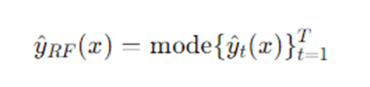
• Classification (majority voting or averaged probabilities):

Majority vote:

Or average class probabilities:

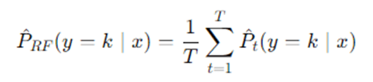
Then pick class ​P RF​(y=k∣x).

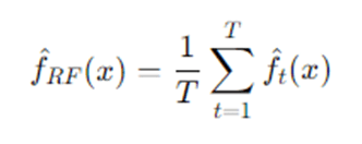
• Regression (average):

Step 5 — Out-of-Bag error estimate

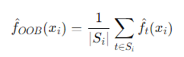
Because each tree is trained on bootstrap sample D_t​, for each observation i we can average predictions from trees where iii was OOB. Let S_i​ be set of trees where i is OOB. Then:

• OOB predicted value for regression:

OOB predicted class for classification: majority vote across t∈Si.

Compute OOB error as average loss across training examples using their OOB predictions (e.g., MSE for regression, misclassification rate for classification). OOB error approximates cross-validation error and is a handy built-in validation.

Step 6 — Feature importance

Two common measures:

1. Mean Decrease in Impurity (MDI): Sum the impurity decrease (e.g., Gini decrease) for each feature across all nodes in all trees where that feature was used, possibly normalized. Roughly:

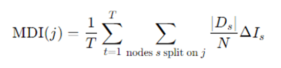
Where, ΔIs is impurity decrease at node s.

2. Permutation importance (Mean Decrease in Accuracy): For each feature jjj, randomly permute its values in the OOB samples, compute the increase in OOB error; larger increases indicate more important features.

Detailed step-by-step explanation

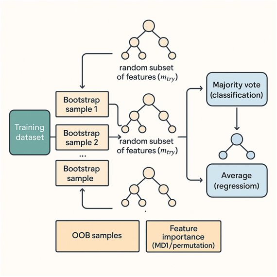
Random Forest begins by accepting the original dataset containing features and labels. Instead of training a single decision tree on all the data, Random Forest constructs many decision trees to form an ensemble. Each tree is grown from a different bootstrap sample — a random sample with replacement from the original dataset — so that each tree sees a slightly different view of the data. Because of sampling with replacement, roughly one-third of the original observations are left out of any given tree’s training set; these are called Out-Of-Bag (OOB) samples and are later used for an internal validation estimate. When a tree is being grown, Random Forest adds another layer of randomness: at each candidate split, the algorithm selects a random subset of features rather than considering all features. This restriction forces different trees to use different variables and prevents a few dominant predictors from controlling every split across the ensemble, increasing the diversity among trees — a good property for ensemble performance.

Each individual tree follows the standard decision-tree splitting logic: repeatedly partition the training subset at each node by choosing a split that maximally reduces impurity (for classification, impurity measures include Gini index or information entropy; for regression, variance reduction is used). Splits are considered only among the randomly chosen subset of features at that node. Trees are typically grown deep and not pruned, because averaging many deep trees reduces variance without the need for pruning; the ensemble prevents the overfitting that a single deep tree would suffer from. Once trees are built, predictions on new data are straightforward: for classification, each tree votes for a class and the Random Forest outputs the majority vote (or averaged class probabilities); for regression, it returns the average of all tree predictions. To evaluate performance without a separate validation set, the model computes an OOB error by testing each training example on the subset of trees that did not use it in their bootstrap training; this OOB error is an unbiased estimate of generalization error similar to cross-validation.

Random Forests provide mechanisms to interpret model behavior. Feature importance can be estimated by tracking how much splitting on a feature reduces impurity across the forest (mean decrease in impurity), or by measuring how much the model’s performance deteriorates when a feature’s values are randomly permuted in the OOB samples (permutation importance). The latter often gives a more reliable sense of feature influence because it measures the feature’s effect on predictive accuracy directly.

Finally, Random Forest models are relatively robust to hyperparameter choices. Increasing the number of trees T typically improves performance (by reducing variance) until returns diminish and computation becomes the limiting factor. The number of features considered at each split (m_try​) controls the bias–variance tradeoff: smaller m_try increases diversity among trees and reduces variance but may increase bias. Other hyperparameters like maximum tree depth, minimum samples per leaf, and minimum samples to split help control overfitting and computational cost.

Example: How Random Forest works ?

Example scenario (classification)

Dataset: Predict whether a patient has disease A (yes/no) using features: Age, Blood Pressure (BP), Cholesterol, Smoking (Yes/No), BMI.

Suppose dataset size N=1000, features p=5. We choose T=100 trees and m_try=5≈2 (so each split considers 2 randomly chosen features).

1. Bootstrap sampling: For tree 1, sample 1000 records with replacement from the 1000 original records; some records repeat, ~368 are left out (OOB) for tree 1.
2. Grow tree 1: At the root node, randomly pick 2 features, say {BP, Smoking}. Among possible thresholds of BP and Smoking splits, choose the one that gives maximum Gini decrease. Continue recursively; each node again selects 2 random features among the 5. Grow until stopping criterion (e.g., minimum leaf size = 5).
3. Repeat: Build 100 trees, each on its own bootstrap and random feature choices.
4. Prediction: For a new patient, each tree returns “yes” or “no.” Suppose out of 100 trees, 73 vote “yes” and 27 vote “no.” Random Forest prediction is “yes” (majority). Class probability estimate: 0.73 for “yes.”
5. OOB error: For record iii in training set, average votes from trees where iii was OOB. Compare OOB majority to true label to compute OOB error rate across the entire training set.

Advantages and disadvantages of Random Forest

Advantages

• High accuracy and robustness: Usually performs well without extensive tuning.
• Reduces overfitting: Averaging many trees reduces variance compared to single trees.
• Handles nonlinearity and interactions: Trees capture nonlinear relationships and interactions automatically.
• Works with mixed feature types: Numerical, categorical, and missing values (with implementations) handled gracefully.
• Built-in feature importance: Gives insight into which variables matter.
• Internal validation (OOB): Gives an unbiased estimate of generalization error without separate validation set.
• Resilient to outliers and noise: Due to aggregation, noisy observations have limited influence.
• Parallelizable: Trees can be trained independently across cores or machines.

Disadvantages

• Less interpretable: The ensemble is a “black box” compared to a single tree; explaining individual predictions is harder.
• Computationally heavier: Many trees can be slow to train and predict (though parallelism helps).
• Memory footprint: Storing hundreds or thousands of trees can consume substantial memory.
• Bias when classes are imbalanced: Might need class weighting or sampling strategies.
• Potentially overfit with noisy data if trees are too deep and too many features correlated: While RF mitigates overfitting, poor hyperparameter choices still cause problems.
• Feature importance biases: MDI importance can be biased toward features with many categories or continuous variables; permutation importance is better but costlier.

Applications of Random Forest

Random Forests are used widely across domains where tabular data is common:

• Finance: Credit scoring, fraud detection, risk modeling.
• Healthcare: Disease diagnosis, survival prediction, medical imaging (as part of pipelines).
• Marketing: Churn prediction, customer segmentation, response modeling.
• E-commerce: Recommendation features, pricing models, demand forecasting (regression).
• Remote sensing / Earth observation: Land cover classification, crop type detection.
• Biology / Genomics: Gene expression classification, biomarker discovery.
• Manufacturing / IoT: Predictive maintenance, anomaly detection.
• Natural Language Processing: Text classification when features are engineered (e.g., TF-IDF).
• Insurance: Claim prediction, risk scoring.

Random Forests also serve as strong baselines for many machine learning tasks — if RF performs well, it can be used in production as a reliable model with moderate interpretability (via feature importance).

Conclusion

Random Forests provide a powerful, flexible, and easy-to-use method for both classification and regression. By combining bagging and random feature selection, Random Forests reduce variance and deliver strong out-of-the-box performance. They’re robust to noise, handle mixed data types, and provide useful internal diagnostics such as OOB error and feature importance. While not as interpretable as single decision trees, they strike a practical balance between accuracy and usability — making them a go-to choice for tabular-data problems and a strong baseline model. For more interpretability, techniques like SHAP values or LIME can be layered on top. For large-scale problems, consider distributed implementations (e.g., Spark MLlib’s RandomForest, scikit-learn with joblib parallelism, or gradient-boosted alternatives if you need higher accuracy at the cost of more tuning).

Frequently Asked Questions (FAQs)

How do I choose the number of trees (T)?

More trees generally reduce variance and improve predictions until a plateau is reached. Typical values: 100–1000. Use cross-validation or monitor OOB error to find diminishing returns; computational budget also matters.

What is max_features (m_try) and how to set it?

max_features is the number of features considered at each split. Default heuristics: classification → sqrt(p), regression → p/3. Smaller values increase tree diversity (lower variance) but may increase bias. Tune if necessary.

When should I prefer Random Forest over Gradient Boosting?

Random Forest often requires less tuning and is more robust to noisy data; it’s a good baseline. Gradient boosting (XGBoost, LightGBM) can yield higher accuracy with careful tuning and is often chosen in competitions, but is more sensitive to hyperparameters. Use RF for quick, stable models; use boosting when you need top predictive performance and can invest in tuning.

How do I interpret feature importance from Random Forest?

Two common methods: Mean Decrease in Impurity (fast but biased towards features with more levels) and Permutation Importance (measures change in accuracy when feature values are permuted; more reliable but costlier). For local explanations, use SHAP values.

Can Random Forest handle missing values and categorical variables?

Many implementations (e.g., some flavors of decision tree algorithms) have heuristics to handle missing values. scikit-learn requires preprocessing for missing values and categorical variables (one-hot or ordinal encoding). Some libraries (e.g., certain R packages or specialized frameworks) support native handling of categoricals and missingness. Consider imputation for missing data or use implementations that support them natively.