
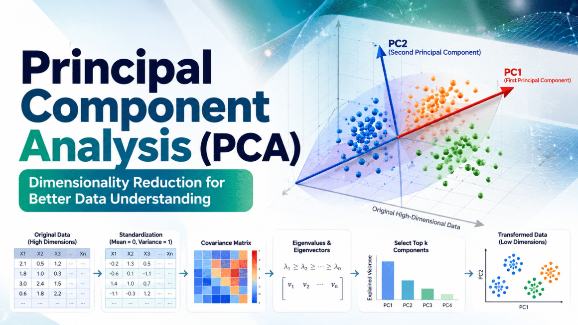
Principal Component Analysis (PCA) is a widely used statistical technique for reducing the number of variables in a dataset while preserving as much of its meaningful variation as possible. It transforms a set of possibly correlated features into a smaller set of new, uncorrelated variables called principal components. This guide explains PCA from its basic idea to its mathematical foundations, algorithmic steps, a worked example, advantages, limitations, and practical applications.
What Is Principal Component Analysis?
Principal Component Analysis (PCA) is an unsupervised dimensionality-reduction method. It takes a dataset containing multiple numerical features and constructs new axes that summarize the data’s variation. The first principal component points in the direction where the data varies most; the second captures the greatest remaining variation subject to being perpendicular to the first; later components follow the same pattern. Each component is a linear combination of the original features.
For example, a dataset may record a student’s mathematics score, physics score, chemistry score, and statistics score. These measurements may be strongly correlated because students who perform well in one subject often perform well in others. PCA can combine related patterns into fewer components, helping analysts visualize the data, reduce storage or computation, and prepare features for other machine-learning models.
PCA does not select a subset of original features. Instead, it creates transformed features. If a dataset has p original variables, PCA can produce up to p principal components, although analysts often retain only the first k components, where k is smaller than p. The resulting representation is compact, but the discarded components may contain information that matters for a particular task.
Introduction to Principal Component Analysis
Modern data often includes many measurements per observation. High-dimensional data can increase computation, complicate visualization, amplify noise, and make some models harder to train. Dimensionality reduction attempts to represent the important structure with fewer variables. PCA is one of the best-known linear methods for this purpose.
The central idea is variance. Variance measures how widely a feature or a direction is spread across observations. PCA searches for a direction onto which the data can be projected with maximum variance. It then searches for another direction that captures the greatest possible remaining variance while being orthogonal to earlier directions. This gives an ordered sequence of components.
Suppose the data points form an elongated cloud in a two-dimensional plot. The cloud is much longer in one direction than the other. PCA places its first axis along the long direction and its second axis perpendicular to it. If the cloud is very narrow across the second direction, projecting onto the first axis may retain most of the variation using a single coordinate.
PCA is unsupervised because it does not use target labels when finding components. It relies on the feature matrix alone. Consequently, components that preserve overall variance do not necessarily preserve the information most useful for predicting a target. PCA is often used as a preprocessing step, for exploratory data analysis, visualization, compression, denoising, and reducing multicollinearity.
Detailed Principal Component Analysis Algorithm
3.1 Notation and data matrix
Let a dataset contain n observations and p numerical features. Represent it as a matrix X of size n × p. The element xij is the value of feature j for observation i. PCA constructs a new matrix of component scores from X. It is important to prepare the features carefully because units and scale can affect the directions found by PCA.
If one feature is measured in thousands and another in fractions, the feature with the larger numerical scale may dominate a covariance-based analysis. Standardizing features is therefore common when their units differ. If all features have the same meaningful scale, centering without standardizing may be appropriate.
3.2 Step 1 — Clean and prepare the data
Begin by identifying the numerical features to include, handling missing values, checking invalid observations, and considering extreme values. Classical PCA generally requires a complete numerical matrix, so missing values may need to be imputed or handled with a method designed for incomplete data. Categorical variables need a suitable encoding strategy if they are to be included; ordinary PCA does not directly operate on text labels or unordered categories.
Let the prepared dataset be X. The rows are observations, and the columns are features. A consistent feature definition is essential because PCA learns its directions from the correlations or covariances present in the data.
3.3 Step 2 — Calculate the mean of each feature
For each feature j, calculate its arithmetic mean across all n observations. The mean of feature j is:
Feature mean
μj = (1/n) Σi=1n xij
Here, μj represents the average value of feature j. Calculate one mean for every column. These means provide the reference point used to center the dataset.
3.4 Step 3 — Center the data (and optionally standardize)
Subtract the corresponding feature mean from every value. The centered value is:
Mean-centering
x′ij = xij − μj
The centered matrix has a mean of approximately zero in each column. This step is important because PCA is intended to describe variation around the data’s center, not variation caused merely by an arbitrary origin.
When features have different units or very different scales, standardize them using each feature’s standard deviation σj:
zij = (xij − μj) / σj
After standardization, each non-constant feature has mean approximately zero and standard deviation approximately one. Constant features have zero standard deviation and must be removed or handled separately. Standardization is not automatically best for every dataset: it gives low-variance features equal initial scale to high-variance features, which may or may not match the problem’s meaning.
3.5 Step 4 — Compute the covariance matrix
The covariance matrix describes how pairs of features vary together. For a centered data matrix Xc, where the rows are observations and columns are features, the sample covariance matrix is:
Covariance matrix
C = (1/(n − 1)) XcTXc
C is a p × p matrix. The diagonal entries contain feature variances, while the off-diagonal entries contain pairwise covariances. Positive covariance means two features tend to move together; negative covariance means one tends to be above its mean when the other is below its mean. A covariance close to zero indicates little linear co-variation, although it does not prove statistical independence.
If standardized values are used instead, the covariance matrix is closely related to the correlation matrix. PCA can be calculated directly from a correlation matrix or from a standardized matrix, depending on the implementation.
3.6 Step 5 — Calculate eigenvalues and eigenvectors
The directions sought by PCA are eigenvectors of the covariance matrix. An eigenvector v satisfies:
Eigenvalue equation
Cv = λv
Here, v is an eigenvector and λ is its corresponding eigenvalue. For a covariance matrix, eigenvalues are non-negative apart from tiny numerical errors. The eigenvector defines a direction in feature space, while its eigenvalue measures the variance along that direction. Because the covariance matrix is symmetric, its eigenvectors can be selected to be mutually orthogonal.
In practice, stable numerical linear-algebra routines should be used to compute the eigendecomposition. The eigenvector’s sign is arbitrary: v and −v represent the same component axis and produce equivalent variance results with the scores’ signs reversed.
3.7 Step 6 — Sort components by explained variance
Sort the eigenvalues in descending order and reorder their eigenvectors in the same way. The eigenvector associated with the largest eigenvalue forms the first principal component (PC1). The next largest defines PC2, and so on. This ordering ensures that the first k components collectively retain the maximum variance possible among k-dimensional linear projections.
The proportion of variance explained by component j is:
Explained variance ratio
EVRj = λj / Σr=1p λr
For the first k components, the cumulative explained variance is:
CEVR(k) = (Σj=1k λj) / (Σr=1p λr)
This value is often used to support a component-retention decision. For example, a researcher might retain the smallest k that reaches a chosen threshold such as 90% or 95%. There is no universal threshold: the appropriate amount depends on the application, validation results, interpretability, and acceptable information loss.
3.8 Step 7 — Select the number of principal components
Choose k components from the ordered set. Common approaches include choosing k by cumulative explained variance, inspecting a scree plot for an elbow, using cross-validation for a downstream predictive task, or imposing a practical constraint on storage and speed. A high explained-variance percentage is useful, but it is not proof that all relevant predictive information has been retained.
If only two components are kept, a high-dimensional dataset can be plotted on a two-dimensional plane. For model training, k may be larger than two if needed to preserve useful structure. Component selection should be evaluated on training data only when working within a predictive pipeline, to avoid leakage from test data.
3.9 Step 8 — Project the data onto the selected components
Place the first k eigenvectors into a loading matrix W, with each selected eigenvector as a column. Project the centered feature matrix into the lower-dimensional component space:
Component scores
Z = XcW
If standardization was selected, use the standardized matrix in place of Xc. The result Z contains n observations and k component scores. Each score is a weighted sum of the original centered or standardized features. Component scores are uncorrelated in the training data under the standard PCA construction, although they are not necessarily statistically independent.
3.10 Step 9 — Interpret and use the result
Inspect the component loadings, explained-variance ratios, and plots of the scores. A loading indicates how strongly an original feature contributes to a component, subject to the convention used by the software. Large absolute loadings can help describe the pattern captured by a component, but interpretation should consider all features and the sign ambiguity of components.
Use the scores as compact features for visualization or downstream modelling. If reconstruction is required, approximate the centered data using ZWT; add the original means back to obtain values on the original scale. With only k components, reconstruction is generally approximate because information from discarded components is not retained.
First, the analyst defines the observations and numerical features that the analysis should describe. Data quality is checked, missing values are treated, and features with no variation are considered for removal. This planning step avoids allowing data-entry errors, arbitrary labels, or uninformative columns to influence the final result. The analyst also determines whether the features should simply be centered or standardized because the units of measurement affect PCA’s geometry.
Next, the mean of each feature is calculated and subtracted from all values in that column. This shifts the data so its center is at the origin. If standardization is appropriate, each centered value is also divided by its feature’s standard deviation. Centering ensures that PCA studies variation around the average observation; standardization helps make features measured on different scales comparable.
The covariance matrix is then calculated from the centered matrix. It summarizes the variance of each feature and how every pair of features varies together. PCA uses this matrix to find new axes that describe the joint spread of the data. When standardized input is used, the computation effectively emphasizes relationships among features after putting them on a common scale.
The algorithm then calculates the covariance matrix’s eigenvalues and eigenvectors, typically with a numerical linear-algebra library. Each eigenvector is a candidate component direction, and its eigenvalue measures the variance along that direction. The eigenvectors are ordered according to their eigenvalues, from the largest to the smallest. The first component therefore captures the largest possible variance along a single linear direction, and each subsequent component captures the greatest remaining variance while staying orthogonal to those already selected.
After ordering the components, the analyst calculates each component’s explained-variance ratio and its cumulative value. These statistics quantify how much of the dataset’s total variance is represented by the first one, two, or more components. A scree plot or a cumulative-variance threshold can help decide how many components to retain, but the final decision should also consider the purpose of the analysis and, where relevant, predictive performance on separate validation data.
The selected eigenvectors are assembled into a projection matrix, and the centered or standardized data is multiplied by this matrix. The resulting component scores represent every observation using fewer numbers than the original features. The analyst can plot the first two scores to explore clusters and outliers, use the scores as model inputs, or reconstruct an approximation of the original data. The complete procedure should be fitted on training data and then applied unchanged to validation, test, and future records in a machine-learning workflow.
Example: How Principal Component Analysis Works
Consider a simple dataset with two standardized-independent measurement features, X and Y, whose centered observations are intentionally arranged along a diagonal pattern. For a transparent numerical example, suppose the sample covariance matrix is:
C = [[2, 1.8], [1.8, 2]]
This symmetric matrix has variance 2 for each feature and positive covariance 1.8 between them. The features therefore tend to increase together. PCA calculates the eigenvalues and eigenvectors of C. For this matrix, the first eigenvalue is λ1 = 3.8 with eigenvector v1 = (1/√2)[1, 1]T; the second eigenvalue is λ2 = 0.2 with eigenvector v2 = (1/√2)[1, −1]T.
The total variance is 3.8 + 0.2 = 4.0. Therefore, PC1 explains 3.8/4.0 = 0.95, or 95% of the total variance, while PC2 explains 0.2/4.0 = 0.05, or 5%. If the goal is a compact one-dimensional representation, retaining only PC1 preserves 95% of the variance in this example. This does not mean every task can safely discard PC2; the low-variance direction might still be useful for a particular target or anomaly.
The first component is the normalized sum direction, so the component score for a centered observation (x, y) is:
PC1 = (x + y)/√2
The second component measures the contrast between the features:
PC2 = (x − y)/√2
Because the observations tend to move together, the sum direction contains most of the variation, while the difference direction contains little. PCA rotates the coordinate system to align with these patterns. By projecting each observation onto PC1, the analyst represents two original values with one score while retaining most of the observed variance.
PCA workflow
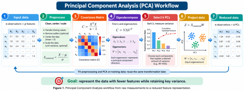
2. PreprocessClean, center / scale
3. CovarianceC = XᵀX / (n − 1) 4. EigendecomposeFind λ and eigenvectors
5. Select k PCsSort λ; measure variance 6. Project dataZ = Xcentered W
7. Reduced datan observations × k PCs Goal: represent the data with fewer features while retaining key variance
Fit preprocessing and PCA on training data; reuse the same transformation later.
Advantages and Disadvantages of PCA
Advantages
Dimensionality reduction: PCA can replace many correlated variables with a smaller number of components, reducing the size of the feature representation and often lowering downstream computation.
Visualization: Converting high-dimensional data to two or three components makes it possible to inspect broad patterns, clusters, gradients, and potential outliers visually. Such plots are exploratory and do not prove that apparent groups are meaningful.
Managing correlation: Principal components are uncorrelated in the data used to fit standard PCA. This can be helpful when original variables are strongly correlated and a downstream method benefits from a more compact representation.
Noise reduction and compression: In some datasets, low-variance components primarily reflect noise. Dropping them can provide a smoother representation and reduce storage requirements. However, PCA cannot reliably distinguish noise from useful low-variance signals without further assumptions or validation.
Deterministic and broadly available: Standard PCA is a well-established linear-algebra method implemented in widely used scientific libraries. Once fitted, the transformation is straightforward to apply to new observations with the same features and preprocessing.
Disadvantages
Reduced interpretability: Each principal component combines original variables, so the resulting feature names may be less intuitive than the original measurements. Loadings can aid interpretation but do not always yield a simple explanation.
Linear method: Standard PCA captures linear directions. It may not preserve curved manifolds or complex nonlinear relationships. Nonlinear dimensionality-reduction approaches may be more appropriate for certain structures, though they come with their own limitations.
Scale sensitivity: Features with large measurement scales can dominate covariance-based PCA. Standardization can address differences in units, but it changes the relative influence of variables and should be chosen thoughtfully.
Variance is not the same as usefulness: PCA maximizes retained variance without looking at a prediction target. A low-variance feature may contain important class or outcome information, and a high-variance direction may reflect irrelevant variation.
Outlier sensitivity: Extreme observations can influence means, covariance estimates, and principal directions. Data quality checks and robust alternatives may be needed where outliers are genuine or frequent.
Information loss: Discarded components cannot generally be recovered exactly. Reconstruction using a limited number of components is approximate, so the retained variance and downstream consequences should be evaluated rather than assumed acceptable.
Applications of Principal Component Analysis
Machine learning and data mining: PCA is used as preprocessing before classification, regression, clustering, and anomaly detection. It can reduce the feature count and help control redundancy, though the value of the transformation depends on the task and model.
Image processing and computer vision: Images can be represented by many pixel values. PCA has been used for image compression, feature extraction, and classic face-recognition approaches such as eigenfaces. Modern deep-learning systems often use other representations, but PCA remains useful for exploratory analysis and compact linear features.
Healthcare and biomedical data: Clinical, genomic, laboratory, and sensor datasets can contain many related variables. PCA can summarize broad patterns and support visualization, quality control, or model preparation. Components should not be treated as clinical explanations or causal factors without appropriate domain analysis.
Finance and economics: Analysts may apply PCA to correlated asset returns, economic indicators, or yield-curve measurements to summarize common movement patterns. Component meanings need to be checked against the data period and methodology.
Text and document analytics: PCA may reduce dimensions after text has been represented numerically, for example through term-frequency or embedding features. For sparse text matrices, truncated singular value decomposition is often a practical related technique because it avoids explicitly forming a dense covariance matrix.
Industrial monitoring and IoT: A system may record readings from many sensors, such as temperature, vibration, pressure, and energy usage. PCA can help visualize operational states, monitor deviations, or reduce redundant sensor dimensions. The detection threshold and model should be validated on representative operating conditions.
Scientific research: In environmental science, biology, psychology, and social science, PCA can summarize correlated measurements and explore dominant variation. Researchers should report preprocessing choices, retained components, variance ratios, and limitations to make the analysis reproducible.
Conclusion
Principal Component Analysis is a foundational technique for exploring and reducing the dimensionality of numerical data. It transforms correlated features into ordered, mutually orthogonal directions called principal components. The algorithm involves preparing and centering or standardizing the data, computing a covariance matrix or performing an equivalent decomposition, sorting components by eigenvalue, selecting an appropriate number of components, and projecting observations into the reduced space.
The worked example shows how a dataset with strongly correlated variables can have 95% of its variance represented by the first component alone. In practical situations, component retention should be guided not only by explained variance but also by the purpose of the analysis, interpretability, and performance on unseen data. PCA is useful for visualization, compression, and machine-learning preprocessing, but it is linear, scale-sensitive, and capable of discarding information. Careful preprocessing, leakage-free evaluation, and transparent reporting help make PCA results more reliable.
Frequently Asked Questions (FAQs)
FAQ 1: What is the main purpose of Principal Component Analysis?
The main purpose of PCA is to reduce the number of numerical features by transforming them into a smaller set of principal components that preserve as much total variance as possible. It is commonly used for visualization, compression, exploratory analysis, and preprocessing for machine-learning models.
FAQ 2: Is PCA a supervised or unsupervised algorithm?
PCA is unsupervised. It learns component directions from the feature values without using target labels. As a result, the directions that preserve the most variance may not be the directions that best separate classes or predict an outcome.
FAQ 3: Why should data be standardized before PCA?
Standardization is often used when features are measured in different units or have widely different scales. It prevents a large numerical scale from dominating a covariance-based analysis. It is not mandatory in all cases; the choice depends on whether the original units and variances should influence the components.
FAQ 4: How many principal components should be retained?
There is no single correct number for every dataset. Analysts may inspect a scree plot, choose a cumulative explained-variance target, or evaluate downstream performance using validation data. A choice such as 90% or 95% explained variance can be a useful starting point, not a universal rule.
FAQ 5: What is the difference between PCA and feature selection?
Feature selection retains a subset of the original features. PCA creates new features as linear combinations of the originals. Feature selection may be easier to interpret, while PCA can represent correlated variation compactly; the better option depends on the task and its interpretability requirements.