What is Glowworm Swarm Optimization Algorithm

The Glowworm Swarm Optimization Algorithm (GSO) is a nature-inspired, swarm-intelligence optimization algorithm that simulates the collective behavior of glowworms to locate multiple optima in multimodal functions. In nature, glowworms emit a bioluminescent chemical called luciferin to attract mates or prey; the brightness tells neighbors something about an individual’s success. GSO models each agent as a glowworm carrying a luciferin level that is increased when the agent finds high-quality solutions and decreased over time. Agents move probabilistically toward neighbors that are brighter (higher luciferin), while dynamically limiting the set of neighbors they consider via a local-decision neighborhood and adaptive sensing radius. The result is a population that can split into subgroups, each converging to different optima — making GSO particularly useful for multimodal optimization and clustering tasks.

GSO was introduced to tackle problems where we want to detect multiple peaks (local and global optima) simultaneously rather than being trapped by a single best solution. Its mechanisms—luciferin update, probabilistic movement, neighbor selection, and sensing-radius adaptation—enable distributed, parallel exploration and exploitation. This makes it an appealing choice in dynamic or multi-solution problems like feature selection, clustering, routing, and multi-modal function optimization.

Introduction of GSO Algorithm

Swarm intelligence algorithms borrow behaviors from biological groups—ants, bees, birds, and fish. Glowworms offer a different metaphor: mobile agents that emit and sense light. A glowworm’s luciferin is a scalar quantity representing local fitness. Agents communicate only locally (within a sensing radius), which results in decentralized decision-making — a major advantage for parallel systems, robotic swarms, and distributed optimization.

A typical GSO run proceeds with a population of glowworms randomly distributed over the search space. Each agent evaluates its fitness (objective function) and updates its luciferin accordingly. Based on neighbors’ luciferin values, agents probabilistically choose a neighbor to move toward. Movement is moderate (controlled step size) to balance exploration and exploitation. Over iterations, agents with high luciferin (better solutions) attract others, forming groups around optima. Simultaneously, agents also explore by moving toward different neighbors or adjusting sensing radius to discover new peaks.

Two central design goals of GSO are:

• Discover multiple optima in the same run.
• Maintain a balance between local refinement (exploitation) and global search (exploration).

Detailed Glowworm Swarm Algorithm

Below is a standard formulation for GSO with common symbols and equations.

Initialization

1. For i=1…n: initialize position x_i(0) randomly within the search space.
2. Initialize luciferin li(0) (a common choice is a small constant or evaluate f(xi(0)) and set li(0) proportional to it).
3. Initialize sensing radii ρi(0) to a constant value (between ρ_min ​ and ρ_max ​).
4. Set parameters: step size s, luciferin decay γ, luciferin deposition coefficient ρ, neighborhood size limit, ρ_min ​, ρ_max ​, radius increment Δ, and maximum iterations T.

Luciferin update

After evaluating the fitness, each glowworm updates luciferin as:

• γ controls how quickly past luciferin decays.
• Ρ scales how much current fitness adds to luciferin.
• If f is to be minimized, set f′=−f or map f to a positive luciferin scale.

Neighbor selection (local-decision domain)

The neighbor set N_i(t) contains agents j satisfying:

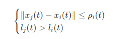
That is, neighbors that are within sensing radius and have higher luciferin.

Movement probability

Given N_i(t) non-empty, the probability of selecting neighbor j∈N_i(t) is:

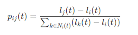
This probability biases movement toward much brighter neighbors.

Movement update

Once a neighbor j is chosen probabilistically, glowworm i moves toward j by:

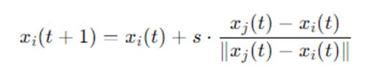
Optionally, if the distance to j is less than s, move to a midpoint or set x_i(t+1) (to avoid overshooting.

Sensing radius (local-decision domain) update

To allow adaptive exploration, update:

• n_t​ is a desired neighborhood size or threshold.

• If too few neighbors are detected, the radius increases; if too many, it decreases. Alternative formulations use:

with signed β direction swapped accordingly.

Termination
Stop when a maximum number of iterations T is reached, or improvement stalls, or the population has stabilized into stable subgroups. The clusters of glowworms represent discovered optima; the positions with highest luciferin in each cluster approximate optima.

Where:

• n: number of glowworms (agents)
• xi(t): position vector of glowworm i at iteration t
• f(x): objective function to maximize (if minimizing, convert by negation)
• li(t): luciferin level of glowworm i at time t
• ρi(t): local-decision (sensing) radius of glowworm i at time t
• N_i​(t): set of neighbors of glowworm i at time t
• s: step size (movement magnitude)
• γ: luciferin decay constant (0 < γ)
• ρ or β: luciferin enhancement factor (commonly denoted γ for decay and β or λ for deposition; we’ll use ρ for luciferin deposition coefficient here to avoid confusion with sensing radius)
• Δ: small positive constant, often used in radius adaptation
• ρ_min​, ρ_max ​: min/max sensing radius
• p_ij(t): probability that glowworm i moves toward neighbor j at time t

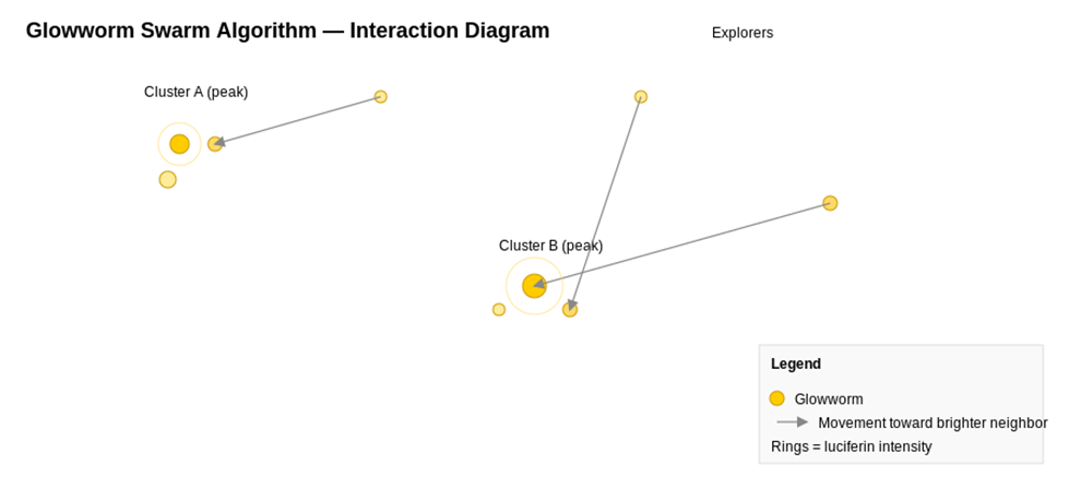
The Glowworm Swarm Algorithm begins with a swarm of glowworms (agents) randomly distributed across the search landscape; each agent maintains a luciferin value representing the attractiveness or fitness of its current location and a sensing radius that dictates how far it can “see” neighbors. During each iteration, every glowworm first updates its luciferin value: the previously stored luciferin decays a bit, then the current objective-function value at the glowworm’s position is added in, scaled by a deposition factor; this dual process ensures luciferin reflects both the recent quality of a location and not just instantaneous noise. After luciferin update, each glowworm identifies neighbors that are both within its sensing radius and have higher luciferin values; this neighbor set is crucial because it restricts interactions to local information, enabling parallelism and preventing premature global collapse. If the neighbor set is non-empty, the glowworm calculates a probability distribution over these neighbors where the probability of choosing any particular neighbor is proportional to the difference in luciferin between that neighbor and the glowworm itself, thereby biasing movement toward much brighter neighbors while still allowing a chance for less bright ones. The glowworm then moves toward a selected neighbor by a fixed step size along the line joining their positions; movement is incremental to maintain stability and allow local refinement. After movement, the glowworm re-evaluates its fitness at the new location in the next iteration, contributing to luciferin updates, and the algorithm also adapts each glowworm’s sensing radius depending on how many neighbors it currently senses — if too few, the radius increases to encourage exploration, whereas if too many, the radius decreases to prevent overcrowding and to foster cluster formation. These interactions produce an emergent behavior where groups of glowworms self-organize around different peaks of the fitness landscape: some groups converge to local optima while others find global ones. Over multiple iterations, luciferin levels stabilize around high-fitness locations and the sensing radius adjustments maintain a balance between exploration (discovering new peaks) and exploitation (refining found peaks). The algorithm stops when a convergence criterion or iteration limit is reached; the final set of glowworm clusters gives the user multiple candidate optima rather than a single best point.

Glowworm Swarm Algorithm (GSO) – Pseudocode

BEGIN GSO

INPUT:
    n = number of glowworms
    T = max iterations
    s = step size
    γ = luciferin decay rate
    ρ = luciferin enhancement rate
    ρ_min, ρ_max = min and max sensing radius
    Δ = radius update constant
    nt = desired neighbor count
    f(x) = objective function (to maximize)

INITIALIZATION:
    For each glowworm i:
        Randomly initialize position xi in search space
        Initialize luciferin li = small positive value
        Initialize sensing radius ρi = ρ_max / 2

FOR t = 1 to T:
    
    # --- Step 1: Luciferin Update ---
    For each glowworm i:
        li = (1 - γ)*li + ρ * f(xi)

    # --- Step 2: Compute Neighbor Set ---
    For each glowworm i:
        Ni = empty set
        For each glowworm j ≠ i:
            If distance(xi, xj) ≤ ρi AND lj > li:
                Add j to Ni

    # --- Step 3: Compute Movement Probabilities ---
    For each glowworm i:
        If Ni is empty:
            continue
        For each j in Ni:
            pij = (lj - li) / Σ over all k ∈ Ni (lk - li)

        Select a neighbor j* according to probability pij
    
        # --- Step 4: Movement Toward Chosen Neighbor ---
        xi = xi + s * ( xj* - xi ) / ||xj* - xi||

    # --- Step 5: Update Sensing Radius ---
    For each glowworm i:
        ρi = ρi + Δ * (nt - |Ni|)
        ρi = max(ρ_min, min(ρ_max, ρi))

END FOR

OUTPUT: Final glowworm positions and luciferin values (estimate of optima)

END

Example of How Glowworm Swarm Algorithm Works

Numerical illustrative example (1D multimodal function)

Consider optimizing the 1D multimodal function:

We want to locate multiple peaks. Suppose we use n=10 glowworms with initial positions uniformly at random. Parameters: γ=0.4, ρ=0.6, step size s=0.1, ρmin⁡=0.1, ρmax⁡=1.0, Δ=0.1, and desired neighbor count n_t=3.

Iteration 0 (initialization):

• Each x_i(0) randomly placed. Evaluate f(x_i(0)) and set:

Some glowworms sitting near actual peaks get higher luciferin. Sensing radius ρi(0)=0.5.

Iteration 1 (luciferin update & neighbor selection):

• Update luciferin:

• For each glowworm, check which other glowworms lie within distance ≤ρi(0)=0.5 and have higher l. Suppose glowworm 3 has two neighbors with higher luciferin; its N3(1) contains those two.
• Compute probabilities p3jusing luciferin differences; choose neighbor j.
• Move: x3(1)=x3(0)+0.1⋅sign(xj(0)−x3(0)) (1D simplification).
• Update ρ3(1) based on number of neighbors: if ∣N3(1)∣<3, ρ3 increases by Δ⋅(3−∣N3(1)∣).

After several iterations:

Glowworms cluster around multiple peaks of f. Those clusters’ centroid positions approximate the peak locations. If two glowworms are at the same peak, their luciferin remain high and they attract nearby glowworms, reinforcing the cluster.

Advantages and Disadvantages

Advantages

• Multiple Optima Detection: Unlike many optimization methods that converge to a single solution, GSO can identify multiple local and global optima in a single run, which is valuable for multimodal problems.
• Decentralized Decision-Making: Agents rely only on local information (within sensing radius), enabling parallelism and robustness to partial failures — appealing for distributed systems and robotic swarms.
• Adaptive Neighborhoods: The sensing radius adapts over time, promoting both exploration and exploitation as needed. This reduces need for delicate parameter tuning in some cases.
• Simplicity and Intuitive Rules: The movement, luciferin update, and neighbor selection rules are conceptually simple and easy to implement.
• Flexibility: GSO can be applied to continuous and discrete problems with appropriate position-encoding and movement operators.
• Robustness to Noise: Since luciferin accumulates over time and decays gradually, the algorithm is relatively robust to noisy fitness evaluations compared with purely instantaneous greedy moves.

Disadvantages

• Parameter Sensitivity: Performance depends on several parameters (luciferin decay γ\gammaγ, deposition ρ\rhoρ, step size sss, sensing radius bounds, Δ\DeltaΔ, desired neighborhood ntn_tnt​). Poor choices can cause slow convergence or missed peaks.
• Scalability: For very high-dimensional problems, local movement with small step sizes can make convergence slow. Additionally, computing neighbor sets for many agents in high dimensions can be computationally expensive.
• Local Trapping: Although the algorithm finds multiple optima, each agent still risks local trapping; proper balance and initial distribution are required.
• No Guarantee of Global Optimum: Like other stochastic algorithms, GSO cannot guarantee finding the global optimum — but it improves chances of finding multiple good solutions.
• Design Choices for Discrete Problems: Applying GSO to discrete or combinatorial problems requires careful design of movement operators; naive mapping can be ineffective.
• Convergence Criteria: Determining when clusters are stable and when to stop can be nontrivial and problem-dependent.

Applications of Glowworm Swarm Algorithm

GSO’s structure lends itself to many areas where discovering multiple high-quality solutions or cluster detection is beneficial. Representative applications include:

• Multimodal Function Optimization: Locating multiple local/global optima in benchmark or real-world functions.
• Clustering and Mode Detection: Using GSO as a clustering method by regarding clusters as attractors in the data space; useful in unsupervised learning tasks.
• Sensor Network Deployment: For robotic or sensor networks, GSO can be used to distribute agents effectively across areas of interest while maintaining local communication and avoiding overcrowding.
• Feature Selection & Subset Selection: GSO can explore multiple good feature subsets in machine learning problems, providing diverse candidate models.
• Mobile Robot Coordination and Exploration: Robots use local signaling and movement rules to explore environments and gather around regions of interest.
• Path Planning: For multi-robot systems needing to explore multiple feasible paths or local solutions.
• Image Segmentation: Clustering pixel-level features into segments by treating luciferin as segmentation quality and letting agents gather around segment centroids.
• Wireless Sensor Networks (WSN): Optimization for clustering nodes and energy-efficient routing by using local signals to form energy-aware clusters.
• Spread-spectrum and Communication Protocol Optimization: Parameter tuning where multiple near-optimal parameter sets are valuable.
• Economic & Game-Theoretic Simulations: Situations that benefit from multiple equilibria discovery.

Because GSO is an exploratory, multi-solution algorithm with local communication, any domain that benefits from parallel, distributed search or discovering multiple candidate solutions is a candidate for adaptation.

Conclusion

The Glowworm Swarm Algorithm is a creative and practical addition to the family of swarm intelligence methods. Its use of luciferin as a local fitness indicator, combined with probabilistic neighbor-based movement and adaptive sensing radii, enables the parallel discovery of multiple optima in complex landscapes. GSO is particularly well-suited to multimodal optimization, clustering, and distributed systems where local decision-making and resilience are important.

While it offers flexibility and an elegant natural metaphor, practitioners should be mindful of parameter choices and computational costs, especially in high-dimensional or noisy environments. For many problems, GSO can serve either as a primary optimizer or as a complement to other methods—providing diverse candidate solutions that can be further refined by local search or hybrid methods.

If you’re dealing with problems where multiple good solutions are valuable (not just one), or if you’re working with distributed agents needing local rules, GSO is worth exploring and experimenting with. Its conceptual simplicity belies a powerful emergent behavior that can be harnessed across engineering, data science, robotics, and more.

Frequently Asked Questions (FAQs)

Is GSO better than Particle Swarm Optimization (PSO)?

GSO and PSO serve different strengths. PSO is excellent at rapidly converging to a single optimum through global information sharing (velocity and neighborhood rules), while GSO is designed to detect multiple optima simultaneously using localized luciferin-based attraction. If your problem is strictly unimodal and you want fast convergence, PSO may be preferable. For multimodal or multi-solution needs, GSO often has advantages.

How do I choose the parameters for GSO (luciferin decay, step size, radius bounds)?

Parameter choice is problem-dependent. Start with literature-recommended values if available (e.g., moderate luciferin decay γ between 0.2–0.6; step size set as a small fraction of the search space diameter), and tune via preliminary runs or automated search (grid/random search). Sensitivity analysis is helpful: vary one parameter at a time and observe cluster formation. Consider adapting step size or using hybrid local search for fine-tuning.

Can GSO be used for discrete optimization problems?

Yes, but movement and distance measures must be redefined. Instead of geometric movement, use neighborhood operators appropriate for the discrete domain (e.g., swap, insertion). Define luciferin based on discrete objective values and neighbor sets based on Hamming distance or problem-specific distance metrics. Careful operator design is essential for good performance.

How does GSO handle noisy objective evaluations?

GSO’s luciferin update incorporates decay and accumulation, which smooths transient noise to some extent. You can further improve robustness by averaging recent fitness evaluations for luciferin updates, increasing decay rate to reduce noise persistence, or adding resampling strategies for uncertain evaluations.

How to detect when GSO has found all relevant optima?

There is no universal stopping rule. Practical approaches include: monitoring cluster stability (no change in cluster centers across iterations), setting a maximum number of iterations, stopping after no improvement in best luciferin values for a number of iterations, or using domain knowledge about expected number of optima. For completeness, you can run GSO multiple times with varied initial seeds to increase coverage of optima.