What is Label Propagation Algorithm?

Label Propagation Algorithm (LPA or LAP) is a simple, fast, and intuitive semi-supervised (and unsupervised) graph-based method for community detection and label inference on graphs. At its heart, LAP treats labels as pieces of information that flow through the network along edges: nodes repeatedly update their label by adopting the label that is most common among their neighbors (optionally weighted by edge strengths). Over a few iterations, labels stabilize and dense regions of nodes share a common label — which naturally corresponds to communities in networks or to inferred labels in semi-supervised tasks. LAP is prized for its near-linear time complexity, minimal parameter tuning, and ease of implementation, which makes it attractive for large graphs where more elaborate inference methods would be expensive.

Introduction of Label Propagation Algorithm

Graph-structured data appears across many domains: social networks, citation networks, recommendation systems, biological networks, and more. Often we want to partition the graph into coherent groups (communities) or infer unknown labels for a subset of nodes given a few labeled exemplars. Label Propagation Algorithm addresses both problems using the same intuitive idea: information (labels) spreads across edges and nodes iteratively reinforce the most prevalent label in their neighborhood.

LAP comes in two main flavors: unsupervised community detection (no ground truth labels; labels are initially unique or random and clusters form when labels stabilize) and semi-supervised label propagation (some nodes are pre-labeled and those labels act as “seeds” to propagate to unlabeled nodes). In the semi-supervised setting, you typically freeze the known labels (they do not change) and propagate them to the rest. LAP gained popularity because it requires few hyperparameters (often none), is embarrassingly parallel in many implementations, and produces meaningful partitions on many kinds of networks.

Conceptually LAP is easy: initialize labels, then repeatedly let each node adopt the most frequent/strongest neighbor label. Mathematically, this can be expressed using label vectors and matrix operations that make the algorithm amenable to analysis and variations (weighted propagation, probabilistic label distributions, normalization, and regularization). In practice, choices such as synchronous vs asynchronous updates, tie-breaking rules, and whether to normalize label scores significantly affect results and convergence.

Detailed Label Propagation Algorithm

Consider an undirected weighted graph G=(V,E,W) with n=∣V∣ nodes. The adjacency (weight) matrix is W={w_ij} where w_ij≥0 is the weight of edge (i,j) (for unweighted graphs, w_ij=1when an edge exists). The degree of node i is d_i=∑_jw_ij ​. Let L be the set of labels used (in community discovery this could be up to n unique labels initially; in semi-supervised learning it is the set of known classes).

Initialization.
We represent the label state as a label indicator matrix F∈R_n×c where c=∣L∣ is the number of label categories. The row F_i,:​ denotes the label distribution at node i. Initialization strategies:

• Hard initialization (unsupervised community detection): assign each node a unique label l_i=i. Then F_i,k=1 if k=l i else 0 (so initially F=I_n or a permutation of identity).
• Seeded semi-supervised initialization: For labeled nodes i∈Si in Si∈S, set Fi,yi=1and for unlabeled nodes set a uniform distribution or zero vector to indicate unknown.
• Probabilistic initialization: initialize F_i:​ to prior probabilities if available.

Formally, let Y be an n×c matrix expressing initial label evidence: Yik=1 if node iii is known to have label k and 0 otherwise (for unlabeled nodes, row zeros). Then initialization sets F(0)=Y or some normalized variant.

Propagation (core update).

At each iteration t, each node i updates its label distribution by aggregating neighbor distributions:

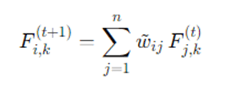
where w~ij ​ are normalized edge weights. Typical normalization choices:

• Row normalization: w~ij=w_ij /d_i (each node averages its neighbors).
• Symmetric normalization: w~ij=w_ij/ d_id_j ​​ (used in spectral methods).
• Column normalization (rare): w~ij=w_ij/ d_j ​​.

In matrix notation:

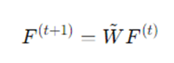
where W~ is the normalized adjacency matrix.

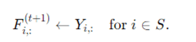
Reinforce known labels (semi-supervised).

If using labeled seeds, after propagation you may want to ensure known labels remain fixed. One way is to reset rows corresponding to labeled nodes:

A soft variant blends propagated distribution with original labels:

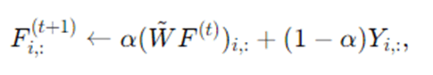
where α∈[0,1] controls how strongly we keep original labels (this is analogous to label spreading / random walk with restart).

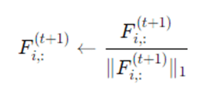
Normalization and discretization.

After propagation, one typically normalizes each node’s label vector to make it a probability distribution:

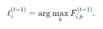
Finally for hard labels, each node picks the label with the highest score:

Convergence criterion.

Stop when labels stop changing (hard labels stabilize) or when ∥F(t+1)−F(t)∥F<ε for some small threshold ε, or after T maximum iterations.

Asynchronous vs synchronous update.

Synchronous update computes F(t+1) from the whole F(t) simultaneously (matrix multiply). Asynchronous update visits nodes in some order and updates them immediately using the most recent neighbor states. Asynchronous often converges faster and avoids label oscillations in some cases, but synchronous is simpler and more amenable to matrix acceleration.

Tie-breaking.
If two labels have equal score at a node, a deterministic tie-breaker (e.g., choose label with smallest index) or random tie-breaker may be used. Tie-breaking affects the resulting partition, especially in symmetric graphs.

Complexity.
A naive propagation takes O(∣E∣c) per iteration (summing over neighbors for each label). For hard label updates, cost reduces to O(∣E∣) per iteration if we only count frequencies. LAP typically converges within small number of iterations (often < 50) on real networks, making it near-linear in |E|.

Detailed step-by-step explanation

Label Propagation begins by preparing the graph representation and the initial labeling state. Suppose we have an undirected graph where edges may carry weights that express the strength of connection between nodes. We store these weights in an adjacency matrix WWW and compute the degree of each node as the sum of weights to its neighbors. To start the propagation process, the algorithm creates a label distribution for each node; in the unsupervised form every node might start with a unique label so that there is maximal diversity, while in the semi-supervised form nodes with known labels receive one-hot label vectors while unknown nodes are initialized neutrally. This initialization encodes prior information: in semi-supervised use the initial labels are the only true ground-truth anchors and they will be preserved or reinforced during propagation.

The heart of LAP is an iterative aggregation step where each node collects label evidence from its neighbors. For a given node, the algorithm inspects the label vectors of all adjacent nodes and computes a weighted sum, where the weight associated with each neighbor can be the raw adjacency weight or a normalized form of it. Normalization—dividing by the node’s degree or using symmetric normalization—ensures the update does not unfairly privilege nodes with extremely high degree. Intuitively, this aggregation means each neighbor casts a vote for the labels it believes applicable, and the receiving node tallies those votes into a score for each label.

Once the scores are collected, the algorithm converts the aggregated scores into a new label state for the node. This conversion often includes normalization to turn scores into a probability distribution, facilitating comparisons across nodes with different degrees. In the simplest, “hard” labeling variant, the node simply selects the label with the largest score and adopts it permanently (for that iteration); in a softer variant the node keeps a probability vector that evolves over time. When seed labels are present, the algorithm makes sure not to overwrite the original labels — either by resetting the labeled nodes to their seed values after each propagation step or by inserting a convex combination step that blends propagated estimates with the original labels, controlled by a parameter that governs label inertia.

A typical iteration is repeated until some stopping condition is met. The most intuitive stopping rule is label stability — when no node changes its label between successive iterations, the system has reached a fixed point and the algorithm halts. Alternatively, one may require the matrix of label distributions to change by less than a small threshold under a matrix norm, or simply stop after a fixed number of iterations chosen empirically. Practical implementations also consider tie-breaking rules: when two labels score equally for a node, the algorithm must decide deterministically or at random which label to choose. Small choices in tie-breaking, synchronous versus asynchronous updates, and whether to normalize scores heavily influence the final partition, so practitioners often test variants to ensure robustness.

The final output of LAP is either a partition of nodes into communities (in the unsupervised case) or a label assignment for previously unlabeled nodes (in the semi-supervised case). Because labels tend to propagate through dense connections, the algorithm tends to group nodes into connected components where intra-group edges are dense. The simplicity of LAP — few parameters, straightforward updates, and direct interpretability — makes it fit well for exploratory analysis and for large networks that need quick, interpretable clustering.

From a mathematical perspective LAP can be seen as performing a repeated multiplication of the current label matrix by a normalized adjacency matrix. This view connects LAP to random walks and diffusion processes on graphs: the propagation step corresponds to one step of a random walk mixing label information across neighbors. When the normalized adjacency matrix is stochastic and the process includes label reinstatement for seeds, the algorithm resembles a random walk with restart, which has well-studied convergence properties. In short, LAP leverages local adjacency structure to spread information, and the repeated linear operations allow it to borrow analysis techniques from spectral graph theory and Markov chains.

Finally, LAP is simple to scale and parallelize: since each node’s update depends only on neighbors, updates for many nodes can be computed in parallel (especially in the synchronous matrix-multiply form). Memory needs are dominated by storage of the adjacency structure and the label matrix. For hard-labeled variants where each node stores only a single label, memory use is small; for soft variants with many possible classes, memory grows with the number of classes c. Because many real problems have small c, this is usually manageable.

Example — How Label Propagation Algorithm works

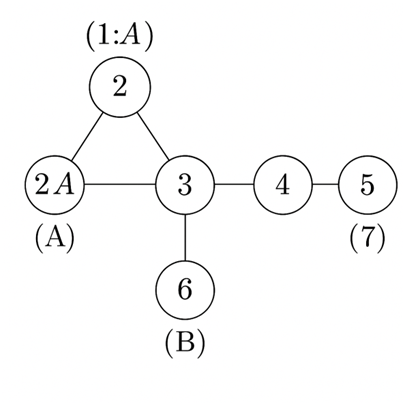
Let us illustrate LAP with a small, concrete example. Consider a tiny undirected unweighted graph of 7 nodes V={1,2,3,4,5,6,7} with edges:

• A triangle among nodes 1–2–3 (edges (1,2), (2,3), (3,1)),
• A chain connecting node 3 to node 4 and then node 4 to nodes 5 and 6 (edges (3,4), (4,5), (4,6)),
• Node 7 connected only to node 5 (edge (5,7)).

Suppose nodes 1 and 2 are initially labeled “A” (seeds), and node 6 is labeled “B” (seed). All other nodes are unlabeled. We want to infer labels for nodes 3,4,5,7.

Initialization sets F₁,:=(1,0) for A/B, F2,:=(1,0), F6,:=(0,1), and other Fi,:=(0,0) (before propagation). We choose simple neighbor averaging, w~ij=1/d_i.

Iteration 1: Node 3 has neighbors 1,2,4. The propagated label scores are the average of label vectors of {1,2,4}—but node 4 is unlabeled initially, so only 1 and 2 contribute and both vote for “A”. As a result node 3 adopts label A. Node 4 sees neighbors 3,5,6. Initially 3 is unlabeled, 5 unlabeled, 6 is B, so node 4 gets a weak vote for B (from 6). Node 5 sees neighbor 4 and 7 (both unlabeled) — no votes initially. Node 7 sees neighbor 5 (unlabeled) — no votes.

Iteration 2: Now node 3 is A and will vote A for 4. Node 6 remains B. Node 4 will receive votes: from 3 (A) and 6 (B) and maybe 5 (still unlabeled); tie may be broken deterministically or randomly. If tie-breaker favors A, node 4 becomes A; if tie-breaker chooses B, node 4 becomes B. Assume node 4 becomes A. Then node 5 sees neighbor 4 (A) and 7 (unlabeled), so node 5 becomes A. Then node 7 sees neighbor 5 (A) and becomes A. Propagation stabilizes with community A capturing nodes 1–5 and 7 while B remains at node 6 — or with different tie-breaking B might capture 4 and 5. This toy example shows how labels diffuse via adjacency and how seeds influence final partition.

Advantages and Disadvantages of LPA

Advantage

• Fast and scalable: Each propagation step involves only local neighbor aggregation, making the algorithm nearly linear in the number of edges.
• Parameter-light: Requires little to no parameter tuning besides choosing a normalization method.
• Easy to implement: Simple operations (neighbor majority voting or matrix multiplication) make it very straightforward.
• Highly parallelizable: Synchronous updates map to matrix multiplications. Asynchronous updates can be performed in parallel across graph partitions.
• Flexible: Works for both: Unsupervised community detection and Semi-supervised label inference (with seed labels)
• Detects dense local clusters: Because propagation is localized, LPA can naturally detect tightly connected communities that global spectral methods might miss.

Disadvantages

• Can be unstable: Small changes in initialization, tie-breaking, or update order can change final results.
• Non-deterministic unless strict ordering and deterministic tie-breaking are enforced.
• Can oscillate — On bipartite or regular graphs, synchronous updates may cause labels to flip indefinitely.
• Biased toward large hubs: High-degree nodes may dominate label propagation, forming overly large communities.
• Struggles with imbalanced classes: Large classes can overwhelm smaller label seeds.
• Local-homogeneity assumption: Works best when connected nodes share similar labels; fails when long-range or feature-based patterns matter.
• Not globally optimized: Since LPA follows local majority rules, it never optimizes a global objective, reducing theoretical guarantees.

Applications of Label Propagation Algorithm (LPA)

• Social Network Analysis: Community detection (friend groups, interest groups). Inferring missing user attributes (interests, political leaning, preferences).
• Citation & Research Network: Clustering papers by topic. Grouping co-authors into research communities.
• Recommendation Systems: Inferring user preferences or item categories from known examples.
• Natural Language Processing (NLP): Semi-supervised lexicon expansion (e.g., sentiment lexicons). Propagating semantic labels across word similarity graphs.
• Computer Vision: Graph-based image segmentation using pixel or superpixel graphs. Label propagation from user scribbles or segmentation seeds.
• Bioinformatics: Annotating proteins or genes from interaction networks. Inferring biological function through neighbor relationships.
• Cybersecurity: Malware clustering using binary similarity graphs. Propagation of trust/reputation in network systems.
• General Machine Learning / AI: Basis for related methods like Label Spreading and Random Walk with Restart. Useful for fast, interpretable bootstrapping before using complex models. Widely used in exploratory data analysis for preliminary clustering.

Conclusion

Label Propagation Algorithm is an elegant, pragmatic method for spreading label information across graphs. From a few simple rules — initialize, aggregate neighbor labels, normalize, and repeat — LAP delivers community structures and label assignments that often align with human intuition and ground truth in homophilous graphs. The algorithm’s strengths lie in simplicity, scalability, and versatility: it requires few parameters, can be applied in both unsupervised and semi-supervised settings, and is trivial to implement for large networks. That said, LAP is not a silver bullet. It is sensitive to initialization and tie-breaking, may produce unstable results on certain graph topologies, and relies on the assumption that connected nodes share labels. Where labels depend on global structure or non-local features, or where robust reproducibility is required, other methods (probabilistic graphical models, spectral clustering, graph neural networks) may be more appropriate. In practice, LAP often shines as an exploratory or bootstrapping tool: use it to quickly understand potential community structure, to generate candidate labels for more powerful supervised models, or to scale-label large graphs when compute resources or labeled data are scarce.

For practitioners, the key levers are normalization choice, update schedule (synchronous/asynchronous), whether and how to preserve seed labels, and tie-breaking strategy. Tuning these thoughtfully — or trying a couple of variants and checking stability — will yield better, more trustworthy results. When applied carefully, Label Propagation is a highly effective, interpretable technique that remains a staple in the graph analysis toolbox.

Frequently Asked Questions (FAQs)

Does Label Propagation always converge?

 LAP often converges on practical networks, but convergence depends on update rules and graph structure. For synchronous updates with hard label discretization, the process will reach a fixed point in a finite number of steps because there are finite label assignments, though it may converge to trivial partitions. In some pathological graphs (e.g., certain bipartite graphs) labels may oscillate under synchronous updates. Asynchronous updates and tie-breaking rules usually help to ensure convergence in practice.

How should I choose normalization (row vs symmetric) for propagation?

Row normalization w~ij=w_ij/d_i averages neighbors and is intuitive; it prevents high-degree nodes from dominating raw sums. Symmetric normalization  w~_ij=w_ij/d_id_j is useful if you want an operation closer to spectral diffusion and to reduce bias from degree heterogeneity. Try both on your problem; symmetric normalization often yields more balanced partitions on graphs with hubs.

How much iteration is needed?

There is no universal answer. LAP often stabilizes in a small number of iterations (e.g., < 20) on real-world graphs. Monitoring the change in labels or label distributions and stopping when changes fall below a threshold is a practical approach. Setting a maximum iteration cap (like 100) prevents rare pathological runs from taking too long.

Can LAP handle directed or weighted graphs?

Yes. For weighted graphs, incorporate weights directly in the adjacency matrix; normalization should account for weighted degrees. For directed graphs, you must decide whether to propagate along outgoing edges, incoming edges, or symmetrize the graph; each choice implies a different semantics for how labels spread. Random-walk interpretations typically use column-stochastic normalization (propagate along outgoing edges).

How does LAP compare to graph neural networks (GNNs) for label propagation?

LAP is much simpler and faster than GNNs and doesn’t require training data beyond seed labels. GNNs can learn complex, feature-aware aggregation functions and capture non-local patterns, often yielding better performance when node attributes matter or labeled data exists for training. LAP is ideal for quick, unsupervised or seed-based labeling; GNNs are better when learning complex label criteria from data is feasible.