What is LightGBM Algorithm?
LightGBM (Light Gradient Boosting Machine) is a high-performance, distributed, and efficient implementation of the Gradient Boosting Decision Tree (GBDT) framework developed by Microsoft. It is designed to handle large-scale data with higher speed and lower memory consumption while maintaining high predictive accuracy. LightGBM belongs to the family of ensemble learning algorithms, specifically boosting algorithms. It builds multiple weak learners (decision trees) sequentially, where each new tree attempts to correct the errors of the previous ones. Unlike traditional gradient boosting frameworks, LightGBM introduces innovative techniques such as:
- Histogram-based learning
- Leaf-wise tree growth strategy
- Gradient-based One-Side Sampling (GOSS)
- Exclusive Feature Bundling (EFB)
These enhancements make LightGBM significantly faster than other boosting frameworks like XGBoost and CatBoost in many scenarios.
Introduction of LightGBM Algorithm
Gradient Boosting Decision Trees (GBDT) are widely used in machine learning for regression, classification, and ranking tasks. However, traditional GBDT implementations face challenges when dealing with: Large datasets, High-dimensional data, Long training time and High memory usage. To overcome these limitations, Microsoft introduced LightGBM in 2017 as an optimized framework for gradient boosting. The core idea behind LightGBM is to improve computational efficiency without compromising predictive performance.
Key Innovations of LightGBM,
- Histogram-based Decision Tree Learning: Continuous features are bucketed into discrete bins, which reduces computation cost.
- Leaf-wise Tree Growth Strategy: Instead of growing trees level-wise (as in traditional methods), LightGBM grows trees leaf-wise by choosing the leaf with maximum loss reduction.
- Gradient-based One-Side Sampling (GOSS): Keeps instances with large gradients and randomly samples those with small gradients.
- Exclusive Feature Bundling (EFB): Combines mutually exclusive features to reduce dimensionality.
Because of these optimizations, LightGBM is widely adopted in industry and data science competitions.
Detailed LightGBM Algorithm
LightGBM is based on Gradient Boosting. Let us understand its mathematical foundation step by step.
Step 1: Problem Setup
Given a dataset:
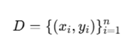
Where:
- xi = feature vector
- yi = target variable
- n = number of samples
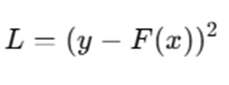
The goal is to build a model F(x) that minimizes a differentiable loss function L(y,F(x)).
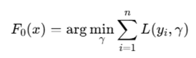
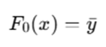
Step 2: Initialize Model
Start with a constant prediction:
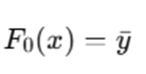
For regression (MSE loss), this is simply:
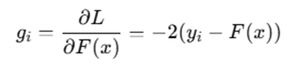
Step 3: Compute Gradients
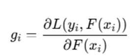
At iteration t, compute first-order and second-order gradients:
First-order gradient:
Second-order gradient:
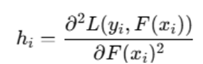
These gradients guide how the next tree should be constructed.
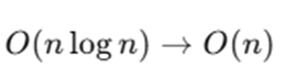
Step 4: Histogram-based Feature Binning
Instead of scanning all unique feature values, LightGBM:
- Divides features into k discrete bins
- Uses histogram to calculate gradient sums per bin
This reduces complexity from:
Step 5: Leaf-wise Tree Growth
For each leaf, LightGBM calculates gain:
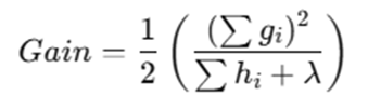
Split gain formula:

Where:
- GL,GR = sum of gradients (left/right)
- HL,HR = sum of Hessians
- λ = regularization parameter
LightGBM selects the split with maximum gain.
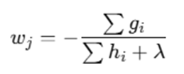
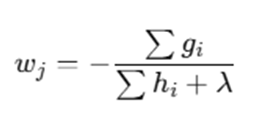
Step 6: Update Leaf Values
Leaf output value:
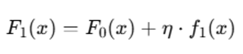
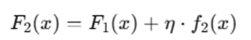
Step 7: Update Model
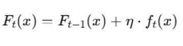
Where:
- η = learning rate
- ft(x) = new tree
Step 8: Repeat
Repeat steps until:
- Maximum number of trees reached
- Convergence achieved
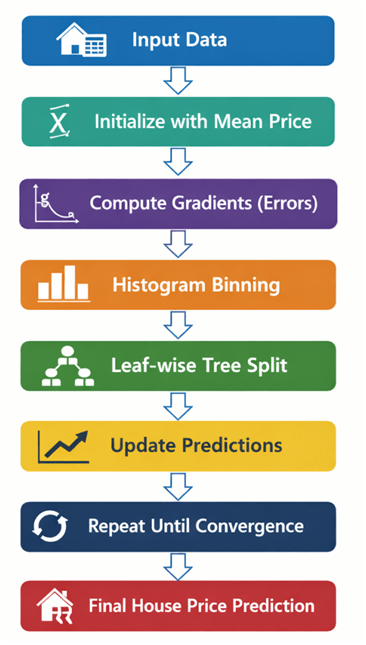
LightGBM begins by initializing the model with a constant value that minimizes the loss function over the dataset. In regression problems, this is usually the mean of the target variable. After initialization, the algorithm proceeds iteratively, building one decision tree at a time. During each iteration, it computes the gradients and second-order gradients (Hessians) of the loss function with respect to the current predictions. These gradients represent how much the model’s predictions need to change to reduce the loss.
Instead of evaluating every possible split value for each feature, LightGBM converts continuous features into discrete bins using a histogram-based approach. This significantly reduces computation and memory usage because the algorithm works with bin indexes rather than raw feature values. For each bin, the sum of gradients and Hessians is calculated, which helps in determining the optimal split point.
Unlike traditional level-wise tree growth used in many boosting algorithms, LightGBM adopts a leaf-wise strategy. In this method, the leaf that yields the maximum loss reduction is split first. This often results in deeper trees and better accuracy, though it may increase the risk of overfitting if not properly regularized. Once the best split is identified using the gain formula, the tree is expanded accordingly. After constructing the tree, each leaf node is assigned an optimal weight based on the ratio of the sum of gradients to the sum of Hessians. This ensures that predictions move in the direction that most reduces the error.
The model is then updated by adding the newly constructed tree multiplied by the learning rate. This learning rate controls how much influence each tree has on the final prediction. The entire process is repeated for a predefined number of iterations or until the model converges. Through this iterative error correction mechanism, LightGBM gradually improves predictive accuracy.
Example of How LightGBM Works
Example: House Price Prediction (Detailed Explanation)
Let us understand how LightGBM works step by step using a practical regression example: predicting house prices based on three features:
- Size (square feet)
- Number of rooms
- Location score (numerical score representing area quality)
Assume we have the following simplified dataset:
| House | Size (sq ft) | Rooms | Location Score | Actual Price (₹ Lakhs) |
| H1 | 1000 | 2 | 6 | 50 |
| H2 | 1500 | 3 | 7 | 65 |
| H3 | 2000 | 4 | 8 | 80 |
| H4 | 1200 | 2 | 5 | 55 |
| H5 | 1800 | 3 | 9 | 90 |
We will walk through how LightGBM builds the model.
Step 1: Initialize Prediction as Mean House Price
LightGBM begins by initializing the model with a constant value that minimizes the loss function.
For regression with Mean Squared Error (MSE):
Calculate mean price:
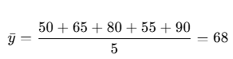
So, initial prediction for all houses:
| House | Actual | Initial Prediction |
| H1 | 50 | 68 |
| H2 | 65 | 68 |
| H3 | 80 | 68 |
| H4 | 55 | 68 |
| H5 | 90 | 68 |
Step 2: Compute Prediction Errors (Gradients)
For MSE loss:
Gradient:
Compute residuals (simplified as y – ŷ):
| House | Actual | Predicted | Residual (y – ŷ) |
| H1 | 50 | 68 | -18 |
| H2 | 65 | 68 | -3 |
| H3 | 80 | 68 | 12 |
| H4 | 55 | 68 | -13 |
| H5 | 90 | 68 | 22 |
These residuals represent how much each prediction is off. LightGBM will build a tree to predict these residuals.
Step 3: Histogram Binning (Internal Optimization)
Instead of evaluating all exact split values for size, rooms, and location score, LightGBM:
- Converts continuous features into bins
- Calculates sum of gradients per bin
- Searches best split using aggregated values
This makes the algorithm computationally efficient.
Step 4: Build First Tree Based on Gradients
LightGBM now builds a regression tree to predict the residuals.
Suppose the best split chosen (based on gain formula) is:
Split on Size ≤ 1400 sq ft
Tree Structure:
Size ≤ 1400?
/ \
Yes No
(-11 avg) (17 avg)
Left Leaf (H1, H2, H4):
Residuals = (-18, -3, -13)
Average = -11
Right Leaf (H3, H5):
Residuals = (12, 22)
Average = 17
Each leaf value is computed using:
(Here simplified as average residual.)
Step 5: Update Predictions
LightGBM updates predictions:
Assume learning rate η=0.1
For left leaf:

For right leaf:

Updated Predictions:
| House | New Prediction |
| H1 | 66.9 |
| H2 | 66.9 |
| H4 | 66.9 |
| H3 | 69.7 |
| H5 | 69.7 |
The predictions move slightly toward actual values.
Step 6: Compute New Errors
Calculate new residuals:
| House | Actual | New Prediction | Residual |
| H1 | 50 | 66.9 | -16.9 |
| H2 | 65 | 66.9 | -1.9 |
| H3 | 80 | 69.7 | 10.3 |
| H4 | 55 | 66.9 | -11.9 |
| H5 | 90 | 69.7 | 20.3 |
Errors are now smaller than before.
Step 7: Build Second Tree (Correcting Remaining Errors)
LightGBM builds another tree using new gradients.
Suppose it splits based on Location Score ≤ 7:
Location ≤ 7?
/ \
Yes No
(-10 avg) (15 avg)
This tree focuses on correcting remaining residual patterns.
Update predictions again:
Predictions get closer to actual prices.
Step 8: Continue Until Model Stabilizes
This process repeats:
- Compute gradients
- Build tree
- Update predictions
- Reduce error
After many iterations (e.g., 100–500 trees), the model stabilizes and predictions closely match actual house prices.
Advantages and Disadvantages of LightGBM
LightGBM is widely adopted in machine learning due to its efficiency and performance. However, like any algorithm, it has both strengths and limitations. Understanding these helps in choosing the right use case and applying proper tuning strategies.
Advantages
- Faster Training Speed: One of the most significant advantages of LightGBM is its extremely fast training speed. This speed improvement comes primarily from its histogram-based learning approach, where continuous features are converted into discrete bins. Instead of scanning all possible split values, LightGBM evaluates splits based on histogram bins, which drastically reduces computational complexity. Additionally, its leaf-wise tree growth strategy selects the leaf with maximum loss reduction, allowing the model to converge faster with fewer trees compared to traditional level-wise boosting methods.
- Lower Memory Usage: LightGBM consumes less memory compared to many other gradient boosting implementations. Since it stores feature values as discrete bins instead of raw continuous values, memory requirements are significantly reduced. This makes it particularly suitable for high-dimensional datasets where memory efficiency is critical. Furthermore, techniques such as Exclusive Feature Bundling (EFB) combine mutually exclusive features, reducing dimensionality and improving memory optimization without sacrificing predictive power.
- High Accuracy: Due to its leaf-wise growth strategy, LightGBM can achieve higher accuracy compared to traditional boosting algorithms. By always selecting the split that provides the highest gain, it focuses directly on reducing loss effectively. The use of second-order gradients (Hessian information) also allows LightGBM to perform more precise optimization. This results in improved predictive performance in both regression and classification tasks.
- Handles Large Datasets Efficiently: LightGBM is specifically designed to work efficiently with large-scale datasets containing millions of samples and thousands of features. Its histogram-based approach reduces time complexity, and distributed learning capabilities allow it to train across multiple machines. This makes LightGBM a strong choice for enterprise-level applications such as fraud detection, recommendation systems, and financial risk modeling.
- Supports Categorical Features Directly: Unlike many machine learning models that require categorical variables to be converted using one-hot encoding, LightGBM can handle categorical features directly. It uses an optimal splitting strategy for categorical variables, reducing preprocessing effort and preventing dimensionality explosion. This feature simplifies data preparation and often improves model performance.
- Parallel and GPU Learning Support : LightGBM supports parallel training across multiple CPU cores and also provides GPU acceleration. Parallel learning allows faster computation during histogram construction and split finding. GPU support further accelerates training on large datasets, making it highly efficient for production-level systems where training time is critical.
Disadvantages of LightGBM
- Can Overfit on Small Datasets : Because LightGBM uses a leaf-wise growth strategy, it can create very deep trees. While this improves accuracy on large datasets, it may lead to overfitting when applied to small datasets. Without proper regularization (such as limiting maximum depth or increasing minimum data in leaf), the model may memorize training data rather than generalize well.
- Sensitive to Hyperparameters: LightGBM’s performance depends heavily on proper hyperparameter tuning. Parameters such as: Learning rate, Number of leaves, Maximum depth, Minimum data in leaf and Regularization terms. Must be carefully adjusted. Poor parameter settings can lead to underfitting or overfitting.
- Complex to Tune: Due to the large number of hyperparameters and their interactions, tuning LightGBM can be complex. Finding the optimal combination often requires: Grid search, Random search and Bayesian optimization. This can increase experimentation time, especially for beginners.
- Leaf-wise Growth May Create Very Deep Trees: Unlike level-wise growth (used in some other boosting algorithms), LightGBM splits the leaf with the maximum loss reduction. While this improves convergence speed and accuracy, it may result in unbalanced trees that grow deep on one side. Deep trees increase model complexity and can reduce interpretability, especially when not properly constrained.
LightGBM offers exceptional speed, efficiency, and accuracy, especially for large-scale machine learning problems. However, it requires careful tuning and regularization to prevent overfitting, particularly on smaller datasets. When properly configured, it is one of the most powerful gradient boosting algorithms available today.
Applications of LightGBM Algorithm
LightGBM is widely adopted across industries because of its high efficiency, scalability, and predictive performance. Its ability to handle large datasets, complex feature interactions, and structured/tabular data makes it particularly suitable for real-world machine learning applications. Below are some of the most important application areas where LightGBM is extensively used.
- Credit Risk Modeling : In the banking and financial services industry, LightGBM is commonly used for credit risk assessment. Financial institutions use it to predict whether a borrower is likely to default on a loan. LightGBM processes features such as income level, credit history, employment status, loan amount, and repayment behavior. Since financial datasets are often large and contain both numerical and categorical variables, LightGBM’s efficiency and support for categorical features make it highly suitable for this task. Its high accuracy helps banks reduce financial losses and improve lending decisions.
- Fraud Detection: Fraud detection systems require fast and accurate prediction models to identify suspicious transactions in real time. LightGBM is widely used in detecting: Credit card fraud, Insurance fraud, Online transaction fraud and Identity theft. Because fraudulent transactions are rare compared to legitimate ones, datasets are often highly imbalanced. LightGBM handles such imbalance effectively using proper parameter tuning and weighted loss functions. Its fast prediction speed is crucial for real-time fraud prevention systems.
- Customer Churn Prediction : Telecommunication companies, subscription platforms, and SaaS businesses use LightGBM to predict customer churn — identifying customers who are likely to discontinue services. The model analyzes features such as usage patterns, billing information, customer complaints, service duration, and engagement metrics.
- Recommendation Systems: LightGBM is used in recommendation engines for e-commerce, streaming platforms, and online marketplaces. It helps predict: Product purchase probability, Click-through rate (CTR), User-item relevance scores. Since recommendation systems often involve large-scale user interaction data, LightGBM’s distributed and parallel training capabilities are highly beneficial. Its ranking objective functions also make it well-suited for learning-to-rank problems.
- Sales Forecasting: Retail companies and supply chain organizations use LightGBM for sales forecasting and demand prediction. By analyzing historical sales data, seasonal patterns, promotions, and external factors (such as holidays or weather), LightGBM can predict future demand accurately. Accurate forecasting helps businesses optimize inventory management, reduce stockouts, and improve operational efficiency.
- Search Ranking: LightGBM is frequently used for ranking tasks, such as search engine result ranking. It supports ranking objectives like LambdaRank, which optimize ordering rather than absolute prediction values. For example, search engines and online platforms use LightGBM to rank: Web search results, Product listings and Advertisement placements. Its ability to handle large datasets efficiently makes it suitable for real-time ranking systems.
- Healthcare Diagnosis: In healthcare analytics, LightGBM is used to predict disease risk, patient readmission probability, and treatment outcomes. It can analyze medical records, diagnostic reports, demographic data, and lab results to assist healthcare professionals in decision-making. Due to its strong predictive capability on structured medical datasets, it is widely used in clinical risk assessment models.
- Stock Price Prediction: In financial markets, LightGBM is applied to stock price forecasting and market trend prediction. It analyzes historical price movements, trading volumes, technical indicators, and macroeconomic variables to predict short-term or long-term price trends. Although stock markets are inherently volatile, LightGBM helps identify patterns in structured financial data and supports algorithmic trading strategies.
Usage in Machine Learning Competitions
LightGBM is extremely popular in data science competitions hosted on platforms like Kaggle. Many winning solutions in Kaggle competitions rely on LightGBM because of: High predictive performance, Fast training time, Flexibility in handling large feature sets and Strong support for ranking and regression tasks. Its competitive edge and scalability make it one of the most frequently used algorithms among professional data scientists.
LightGBM has become a preferred algorithm across industries including finance, healthcare, retail, and technology. Its speed, accuracy, and scalability enable it to solve complex predictive problems efficiently. Whether used for classification, regression, or ranking tasks, LightGBM consistently delivers strong performance in both research and real-world production systems.
Conclusion
LightGBM has established itself as one of the most powerful and efficient gradient boosting frameworks in modern machine learning. Developed by Microsoft, it was specifically designed to address the computational limitations of traditional Gradient Boosting Decision Tree (GBDT) algorithms. By integrating innovative techniques such as histogram-based learning, leaf-wise tree growth, Gradient-based One-Side Sampling (GOSS), and Exclusive Feature Bundling (EFB), LightGBM achieves remarkable improvements in both speed and memory efficiency without sacrificing predictive performance. One of the primary reasons behind LightGBM’s popularity is its ability to scale efficiently. In real-world industrial applications, datasets often contain millions of records and thousands of features. Traditional boosting frameworks may struggle under such conditions due to high computational complexity and memory requirements. LightGBM overcomes these challenges by converting continuous features into discrete bins, significantly reducing the cost of split finding. This design allows it to train faster while consuming less memory, making it suitable for large-scale enterprise systems. Another defining characteristic of LightGBM is its leaf-wise growth strategy. Unlike level-wise tree construction used in some other boosting algorithms, LightGBM expands the leaf that provides the maximum reduction in loss. This strategy often results in better accuracy because the algorithm focuses directly on the most significant errors at each iteration. However, this advantage also introduces the need for proper regularization to avoid overfitting, especially when working with smaller datasets.
LightGBM is versatile and supports multiple learning objectives, including regression, binary classification, multiclass classification, and ranking tasks. Its built-in support for categorical features reduces preprocessing complexity and prevents unnecessary dimensional expansion. Additionally, parallel learning and GPU acceleration make it highly suitable for time-sensitive machine learning workflows. Despite its strengths, LightGBM requires thoughtful hyperparameter tuning. Parameters such as learning rate, number of leaves, maximum depth, and regularization coefficients must be carefully selected to ensure optimal performance and generalization. When properly configured, LightGBM consistently delivers state-of-the-art results across various domains including finance, healthcare, marketing, and e-commerce.
As machine learning continues to evolve toward larger datasets and more complex predictive problems, LightGBM remains a critical tool for data scientists, AI engineers, and researchers. Its balance between computational efficiency and predictive power ensures that it will continue to play an important role in both academic research and industrial applications.
Frequently Asked Questions (FAQs)
Is LightGBM better than XGBoost?
LightGBM is generally faster and more memory-efficient than XGBoost due to its histogram-based binning and leaf-wise growth strategy. In large-scale datasets, LightGBM often trains significantly faster while achieving comparable or better accuracy. However, the overall performance depends on dataset characteristics, hyperparameter tuning, and the specific problem being solved. In some smaller datasets, XGBoost may perform equally well or even better depending on configuration.
Does LightGBM support categorical variables?
Yes, LightGBM natively supports categorical features. Unlike many algorithms that require one-hot encoding, LightGBM can directly handle categorical data using an optimized splitting strategy. This reduces preprocessing time and prevents the curse of dimensionality that may arise from one-hot encoding, especially when categorical variables have many unique values.
Why is LightGBM faster than other boosting algorithms?
LightGBM is faster primarily because of two design choices:
- Histogram-based binning: Continuous features are grouped into discrete bins, reducing the number of split evaluations.
- Leaf-wise tree growth: Instead of expanding trees level by level, LightGBM grows the leaf with maximum loss reduction, allowing faster convergence.
Additionally, parallel processing and GPU support further accelerate training.
Can LightGBM handle large datasets?
Yes, LightGBM is specifically designed for large-scale data. It performs efficiently with millions of samples and high-dimensional feature spaces. Distributed training support allows it to scale across multiple machines, making it suitable for enterprise-level big data applications.
Is LightGBM suitable for small datasets?
LightGBM can work effectively on small datasets; however, due to its leaf-wise growth strategy, it may overfit if not properly regularized. To prevent overfitting, practitioners should:
- Limit the maximum depth
- Reduce the number of leaves
- Increase minimum data in leaf
- Apply regularization parameters
With proper tuning, LightGBM can still deliver strong performance even on moderately sized datasets.